Modeling and Predicting the Impact of Climate Variability on Influenza Virus Spread in Cuba
Influenza viruses are among the main causes of acute respiratory infections in Cuba, associated to pneumonia, and among the five first causes of dead in the last decades. Tropical climate has a great influence on influenza variations and seasonality. The significant increasing of climatic anomalies yield by anthropogenic climate change, carries modifications in the reproductive capacity of the virus and its circulation in temporal as in spatial scale. That´s why, forecast the dynamic of influenza in the country, would allow to health system decision-makers taking the appropriate actions to control the disease.
Introduction
Influenza is the most contagious of the acute respiratory infections (ARI) and influenza viruses are their etiologic agents [1]. These viruses are characterized by a great antigenic and genetic variability affecting its superficial proteins (Hemagglutinin and Neuraminidase). This property provokes its continuous circulation in human population, propitiating the emergence of new antigenic variants that escape from the immunity induced by natural infections and vaccines. This mainly happens due to accumulation of punctual mutations in genes codifying to Hemagglutinin and Neuraminidase [2]. The new viral variants are introduced in the people with no immunity and may yield epidemics or pandemics because of the wide susceptibility to them. This provokes not only thousands of dead people worldwide, but also millionaire lost in production, increasing of health expenses, and labor and school absences [3]. This situation could be similar in Cuba, which has universal health coverage and a high percentage of people involved in both sectors (Productive and Health). That justifies the need of obtaining models to forecast and early warning of viral circulation.
In 2000, the Ministry of Public Health in Cuba (MINSAP) approved and implemented the National Integral Program for Prevention and Control of ARI, whose main objective is to reduce the ARI mortality and morbidity in Cuban population [4]. Particularly, important efforts have been performed to minimize the impact of influenza disease. Every year, the MINSAP invests around 1,2 million USD in acquiring the necessary seasonal flu vaccines to immunize pregnant women, children, elderly≥85 y.o., all institutionalized elderly and people at risk, among them health care workers and those working in avian and swine farms [4]. Influenza viruses present different patterns according to the climate. Several studies report the maximum viral circulation in temperate climates during winter season [5, 6, 7, 8, 9]. In tropical climate regions the maximum viral circulation is during rainy and warm season, especially associated to humidity, temperature and precipitations [10, 11, 12, 13, 14, 15]. The temperate climates patters have been better studied and characterized than in tropical climates, as in the Cuba. Recent studies have allowed to-establish the seasonality of influenza viruses in the country, during the rainy season May – October, with a high association with climate variations. There has been also described its temporal and spatial pattern, no lineal and heterogeneous, according to climate conditions of each region [16, 17, 18].
These viruses develop well in conditions of high temperatures, high humidity and low pressures, which characterize their seasonal and spatial patterns with an additional effect. The Cuban climate characteristics, joined to pH changes in the respiratory tree and the acidification of the epithelial lining of airways, favor the infection in humans [18].
Generally, the models used by other authors to predict those virus circulation, as the Autoregressive Integral Moving Average Exogenous model (ARIMAX), as well as the Iterative Generalized Least Squares-autoregressive model of order p (IGSL-AR(p)) [19, 20], have two limitations. The first one: they only use climate elements as temperature and humidity in an independent way to explore the association with the increasing of influenza virus circulation [20, 21]. The second limitation: they assume that information should has constant mean and variance with absence of heteroscedasticity, which is little probable in real conditions. Those models don´t analyze the climate in its complexity, neither considering the heterogeneity due to the change in the variance, both in the climate as in the virus’s series, for the contrary of the models presented in this work.
Based in the previous findings, in this study two models of no constant variance are developed allowing to simulate and forecast the spatial and temporal distribution of the influenza viruses’ activity associated to the seasonal climate variability with a complex approach, taking in consideration several climate elements. It is also showed the climate variability as an indicator describing the favorable conditions or not, for the viral circulation and its future dynamic with up to three months in advance.
Methods
Design
Ecologic study with retrospective-prospective analysis of influenza series and the climate anomalies described by Bultó climate indexes in the period 2010-2020. To spatial structure, the serial data interpolated from 10km weight matrix was used by Kriging method. An ecologic study with retrospective-prospective analysis of non-lineal influenza series, combined with spatial analysis was performed. For the model´s formulation and fitting, the period 2010- 2014 was taken. To evaluate its performance or predictive value, the period 2015-2016 (independent simple) and the implementation in real time was during the period 2017-2020. Due to space reasons, this text just shows the validation of spatial modelling for some months of the rainy season (June-September, those of higher virus circulation in Cuba) and for the less rainy season the month with minor circulation (January) in 2016. To illustrate the real time temporal forecast, the quarter April-June 2020 was taken. It is also shown as example the spatial outcome for April 2019 (transition month to the rainy period) which allowed formulating in the moment previsions on the possible advance in the start of the virus activity.
Study Area
The Republic of Cuba is located in the so called American Mediterranean, between 19o 49’ and 23o 11’ of north latitude; 74o 08’ and 84o 57’ of west longitude. Its climate is tropical with a rainy season in summer and other less rainy during winter, according to Köppen classification. The main annual temperature varies from 24oC to 26oC and is higher in the coasts. The is seasonality in the thermal regimen with two periods: the rainy period (May to October, with July and August as the warmer months) and the other, in the less rainy (November to April with January and February as the coldest). Annual precipitation is 1335 mm and is associated to tropical cyclones, cold fronts, local storms, tropical waves or convective processes [22, 23].
Variables
Climate Data
The monthly series are composed by the values of Bultó indexes (BI1,t,c) which were built with the following variables: maximum and minimum mean temperature, precipitation and number of days with precipitation, relative humidity, atmospheric pressure, water vapor, thermic oscillation, among others [24]. The climatic series were obtained from the 64 meteorological stations of the Institute of Meteorology, covering all the country during the period 2010-2020. The (BI1,t,c) takes values from negative anomalies (-0.75; -3) of less rainy period November-April and positive anomalies (0.75; 3) of rainy period May-October. April (0; -0.75) and May (0; 0.75) are transition months [24, 25].
Epidemiological Data of Influenza
45,000 clinical samples (nasal swab, nasopharyngeal swab and pharyngeal lavage) were processed from the different provinces of the country. Up to 10,800 (24%) resulted positive to Influenza A and B viruses. Patients of any age with acute infection in the upper or lower respiratory tract, with no more than three days since the onset of symptoms, who expressed written consent for sample taking, were included in the study [17] with the data conforming the temporal series, allowing calculating the monthly virus positivity at provincial level: Proportion of influenza positive samples during the month=Total of positive sample by province during the month/Total of positive sample in the country during the month X 100 [26].
Interpolating Method to Spatial Structure
To this analysis, several techniques of spatial statistic developed in three stages were implemented. The first one consisted in generate a grill with continuous information from 600 nodes (raster format); it means, to transform the information of a finite number of samples in a continuous space, allowing to know the variation pattern in the area, being comparable with that observed in the studied sample [18], as well as characterize areas where there is not information available. For that, the Kriging method combined with the method of inverse distance (IDW) was implemented with the goal of interpolate, to a 20km2 resolution, counting with information in all the studio dominium [27, 28, 29, 30, 31].
The calculation of the Moran coefficient of spatial autocorrelation was predetermined to a neighbor matrix (Queen method) with the information of cases in a radio of 10kilometers, which is the maxim distance to with all the observations had at least one neighbor [18]. Both climatic and viral information (influenza positive cases) were geo-referenced taking in account its location in the geographic space. The political-administrative distribution is a geographic clipping (location recognizable by political decisions) contributing to visualize the grill points to its better comprehension, and allowing to observe the geographical points distributed in a study area (provinces).
Models of Temporal Proceedings
To simulation and prediction of influenza, an analysis of no lineal heteroscedastic time series was performed taking in account the climate variability, and autoregressive models with exogenous variables were elaborated [26, 32].
Models of Autoregressive Conditional Heteroscedasticity (ARCH)
The ARCH effect is referred to a relation within the heteroscedasticity, named serial correlation of heteroscedasticity. Frequently, it´s evidenced when there is an accumulation in the variance or variability of a variable in particular, generating a pattern determined by any factor (the climate in this case). The proportion of influenza positive cases with variability (epidemic pics of the series) was used to represent the epidemic risk [17], and it was assumed that the ARCH effect measured the epidemic risk, given the following model:
u X Y
+ + = β β
1 0 t t t u N u ---------- (1)
) ,0 ( ~ 2 1 1 0
− + α α t t Where Yt: is the dependent variable, βo: is the constant or model level Xt: is an independent variable, and ut is the error term.
This model suggests that the error term is normally distributed with a mean cero and a conditional variance that depends on the squared error term, delayed one-time period. Then, the conditional variance of the error term delayed K times is given by:
) , \ ( ....) , \ var( 2 1 2 2 1 2 − − − − = = t t t t t t t u u u E u u u σ ----- (2) Where 2 t σ is the conditional variance of the error term of ut and the ARCH effect is modelled by:
2 1 1 0 2 − + = t t u α α σ ----- (3)
Where 2 t σ is the variance, α0 is the constant, α1 the parameter, ut is the error term This is the ARCH model (1), then only contain a lag in the squared error term; however, it is possible to extend it to any number of lags, if have got q lags, then it is named ARCH model (q). The expression (3) could be modified by an exogenous term, whether it is assumed that the variance is modulated by an external factor like the climate. Then, the previous expression could transform in:
2 π α µ α σ + + = − ----- (4) Where BIt,r,c, represents the Bultó index used in this study, which describes the behavior of climate variations [25, 31], favoring or not the increasing of variability and then, the influenza epidemic risk. From the previous, an Autoregressive Conditionally Heteroscedastic Exogenous Model (ARCH-) is obtained [19, 20, 32].
2 BI c r t t t , ,
1 1 0
Diagnostic of Predictor by Granger Causality Test
To introduce a predictor variable in the multivariate models of time series, it should be determined if the series are useful or not to allow the forecast of another variable. If Ho is rejected, the climate index is a good predictor according to the Granger causality test [33], to explain the dynamic of influenza viruses and their outbreaks.
To confirm the assumption of autoregressive heteroscedasticity, the Breusch-Godfrey contrasts (explain the evolution of explicative variables with their variance and co-variances), the Lagrange multiplier (LM), the White test and the Lagrange multiplier test to the ARCH LM-ARCH model were used [20, 34, 35, 36, 37]. Simulation of time-based behavior was made by no lineal models with changing variance (ARCH) and with exogenous variables. To prove the model fitness, the Durbin Watson statistic, the criteria of Akaike and Schwarz (this last one to optimize the model selection according to criteria of minimum information), as well as the contrast of Engles and Ljung-Box were used [20, 31, 32, 38].
General Model of Spatial Ponderation
To simulate the spatial series of viral activity, it was considered that its spatial distribution is characterized by a strong spatial correlation [18]. The spatial model used was [28, 39]:
1 1 t t t y Wy X u ρ β − − = + +
2 1 t t u W u λ ε − = + -------- (5)
ε~N(0,Ω) Where, y is the vector (nx1) of the dependent variable observations (influenza virus), ρ is the autoregressive coefficient, Wy is the vector of independent variables pondered by the matrix W of neighbor observations in the time t-1, β is a vector of 1 nx dimensions of the parameters associated with the exogenous variables (it means, spatial lag) in the matrix X of dimension 1 nx (which describes the dynamic of the climate variations due by the BIs in the time t-1),λ is el coefficient of the autoregressive spatial structure to the error u , ε is the sample error.
The matrix of spatial weighs W was calculated using the spatial weighs by distance between neighbors (geo- referenced point with a 10km radio, obtaining the higher spatial autocorrelation). The influence of influenza virus´s circulation in the bordering areas, depends more from the distance between them, than in the areas shape and size [40, 41, 42].
Description of the Spatial Model
Once identified the existence of spatial autocorrelation and given that these models are calculated by the method of maximum plausibility, spatial correlation tests were performed, applying the Moran I and the Lagrange multiplier (LM) tests to the rests of the ordinary minimum square model (MCO): Lagrange multiplier test to the lags (LM- lag), Lagrange multiplier test to the error (LM-error), and the robust to LM Lag and LM-Error. To select the better model of spatial autocorrelation and the description of its structure (spatial lag model of the variable or spatial lag model of the disturbances), where just one of the tests is significant, the model that reject the null hypothesis of no spatial autocorrelation was selected. If both of them were significant, then the robust forms were considered; if just one of the robust statistic was significant, that model was selected, but if both were significant again, the model with the higher statistic value was selected [18, 28, 43]. In this study, it corresponds with the spatial regressive mix models with autoregressive and heteroscedastic disturbances, depending on the case [28].
Measures to Evaluate the Quality of the Models Tight to the Forecast
To evaluate the predictive capability during the test period (2015-2016) several metrics were used before to application the model (period 2017-2020): the absolute mean error (AME), the quadratic mean error (CME) and the bias that could be positive when the model overestimates the prognostic value regarding the real value, and negative when underestimate it, combined with the concordance index Di and the Skill Factor [44, 45, 46]. Precision is understood as the degree of concordance between pairs of individuals from the forecasted values and the observed values in the influenza series, so in a monthly scale as in point to point in the spatial item, considering that the model is appropriate when it reaches values over 70% of concordance.
The results of the spatial models were represented by thematic maps of the country, showing the expected spatial distribution of the influenza virus dynamic for each one of the seasonal periods forecasted, as well as the forecasts with the expected configurations.
Processing the Information
To do the fit and run of the temporal models, the program EViews7 version 2010 was used; to the spatial models the software S-Plus 8.1 on Windows and the Open GeoDa0.1.4.6 version 2017 were used. The parameters of the models were considered statistically significant when p < 0.05. The software ArGis 10.1 was used to built the maps.
Result
Sensibility of the Influenza Viruses to the Seasonal Climate Variations
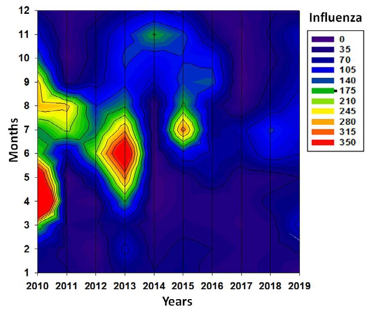
Figure 1 shows the circulation of influenza viruses with different behaviors every year. It is also appreciated a changing monthly viral circulation whose maximum values occur between May and October, the most humid and warm period in the year; meanwhile, in the coolest and driest months (dry period) a decreasing in the virus circulation is shown. That shows the influence of climate and the sensibility of virus circulation to that variability’s.
Diagnostic to Select the Model and its Structure for the Influenza Virus Prediction at a Temporal Scale
An autoregressive model of two orders was selected, with exogenous variables and a heteroscedastic component, because in the Ljung-Box test the first and second lag was significant for p≤0.05 with values 0.637 and 0.272 respectively. Besides, with criteria of minimum Akaike and Schwarz, with values of 10.36 and 10.42, and a likelihood function of -428.12 with a statistic F=59.54 significant to 95%. The Durbin Watson test was 1.596 (p<0.01). The Breusch-Godfrey-LM statistic was significant with value of 39.75, corroborating the presence of explicative variables. Meanwhile, the White and ARCH statistics, both also significant with values of 87.86 and 0.09, respectively, confirmed the presence of a non- lineal autoregressive structure with exogenous variables; it means a model like AR (p)-ARCHX (q). The Granger causality test show values of 5.53 for the first lag and 3.69 for the second, both highly significant. So, the climatic indexes were included as exogenous variables with a memory of one and two months respectively.
The tests on the rest´s squared show that their variance changes with an autoregressive pattern. From the diagnostic results, the use of combined models like AR (p)-ARHC (q) is induced, corroborating the hypothesis for the formulation of regressive models with temporal dependence and heterogeneity by groups, to simulate the transmission of seasonal influenza [21]. In this study, changes in volatility or variance are not used explicitly, as indicated by another authors [2e].
In this research, it was corroborated that climate variability influences the dynamic of influenza virus series, since the seasonal relationship of both was verified. This creates favorable conditions for viral presence and circulation and the need of include the climate seasonal variability in the model as exogenous variable. Similar results were already reported by other researchers [18, 21, 26].
Parameter of the Temporal Model with Exogenous Variables
Table 1 summarizes the results of parameter´s estimations for both temporal and spatial models to influenza viruses. A combination of AR (p)-ARCH (q) with exogenous variables (the descriptor indexes of climate variations) was identified. All the parameters are significant and feasibility is evidenced, because they obtain the lower values in the Akaike and Schwarz criteria, and an adequate fit quality for the temporal model proposed to predict the temporal dynamic of influenza virus. In the spatial scale, the parameter values of the more plausible model are also shown, resulted from adjustment of the autoregressive model, where all parameters identified were significant and their errors were small.
Variables model Coefficients Std. Error z-Statistic Pr(>|Z|) Constant 29.74776 1.966027 15.1309 0.0000 BI1,t,predict (-1) 7.568908 1.073576 7.05018 0.0000 AR(1) 0.657228 0.040815 16.1024 0.0000 AR(12) -0.08716 0.021652 -4.02541 0.0001 Variance Equation Constant 76.0349 25.00535 3.04075 0.0024 ARCH(1) 2.605108 0.476427 5.46801 0.0000 BIt,2,Predict 197.3057 58.33343 3.38238 0.0007 Summary of the AR(p) X ARCH (q) model fitting parameter R-squared: 0.79575 Akaike info criterion 9.155648 Schwarz criterion 9.378729 Log likelihood -318.0255 F-statistic 10.48686 Durbin-Watson stat 1.941971 Prob(F-statistic) 0.0000 Coefficient of the Spatial Autoregressive Model (SAR), with spatial resolution 10km and main statistic to Influenza Variables model Coefficients Std. Error z-Statistic Pr(>|Z|) ρWInf 0.941839 0.015202 61.9538 0.00000 Constant 0.05264 0.160086 1.43288 0.027429* longitude 0.008879 0.003258 2.72527 0.00643 latitude 0.017253 0.008774 1.96641 0.04925* BI1,t,predict 0.395649 0.097834 3.02193 0.00251 Spatial effect (Rho) 0.941839
- Likelihood Ratio Test
- 483.595
- 0.0000**
- Summary of the SAR Model Fitting Parameter
- R-squared:
- 0.922496
- Legend: *p<0.05 ** P<0.01
- Log likelihood
- -225.982
- Akaike info criterion
- -441.963
- Schwarz criterion
- -444.179
Table 1: Summary of AR (p) x ARCH (q) model-Spatial Autoregressive Model (SAR) to simulate and predict Influenza from
Quality of the Viral Circulation Forecasts of the Integrated Model AR (2)-ARCH (2)
The values of the quality indicator for the temporal model are high, because the Skill (βi) and concordance (Di) factors are 0.951 and 0.960 respectively, with an ECM of 2.64 and an EMA of 2.77, predominating a positive bias (2.63) to the proof period of the model (2015-2016). That´s why the model became appropriate to simulation and prognosis of influenza virus circulation in the country since climatic conditions.
Seasonal Forecast of Influenza
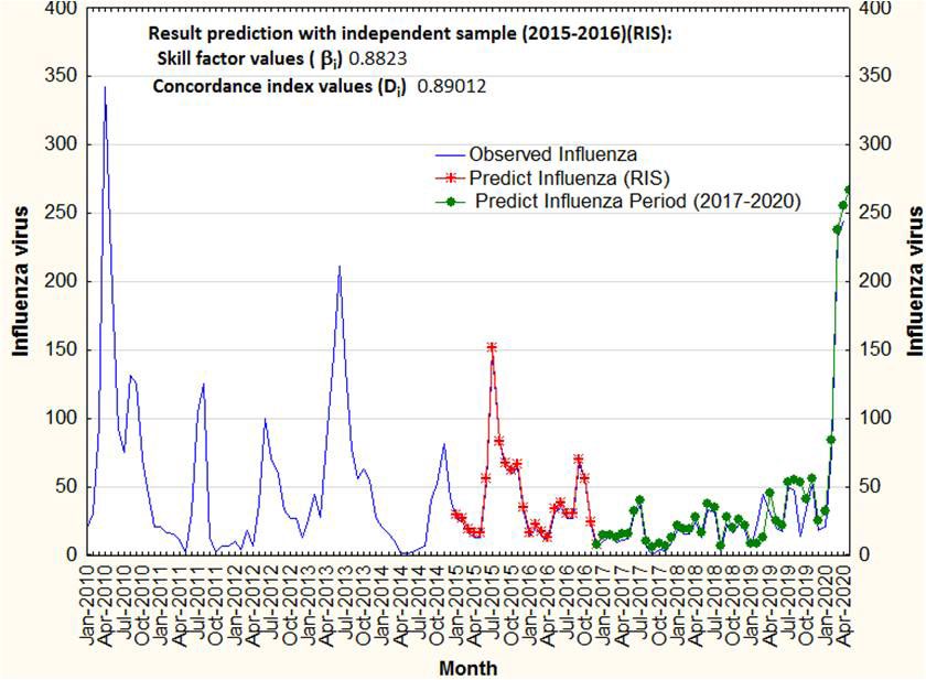
Figure 2 shows temporal dynamic of the series observed between 2010 and 2020, the forecast with independent sample for the period 2015-2016 and the proof period in real time since 2017 to 2018, as well as the seasonal forecast for January 2019 - April 2020. It’s corroborated that large epidemics occur every two years, as well as that the adjusted model with Independent samples presents stability when compared with the validation results with the sample in real time, showing that the forecast errors that are reached are minimal and that the model can simulate and predict epidemic peaks.
Diagnosis to Selection of Spatial Model
The Moran index for the influenza series was 0.881, with Z=12.163 highly significant (p<0.001). A strong spatial correlation between neighbor points was evidenced. The multivariate Moran I was also significant (0.791) with Z=10.1 (p<0.05), proving the climate influence on the virus spatial pattern. The Lagrange multiplier test with lag was 9.23 (p<0.01) and the robust test of Lagrange multiplier with lag was 7.21, also highly significant <0.001), which indicated the presence of an autoregressive spatial dependence model with exogenous variable. The tests for errors were no significant.
Quality of the Proposed Spatial Autoregressive Model (SAR)
The proposed model (Table 1) results appropriate for the simulation of viral circulation at spatial scale in the country; for that reason, its capacity to predict the spatial comportment according to the climate behavior was determined.
Predictive Capability of the SAR Model with Seasonal Climatic Forecasters
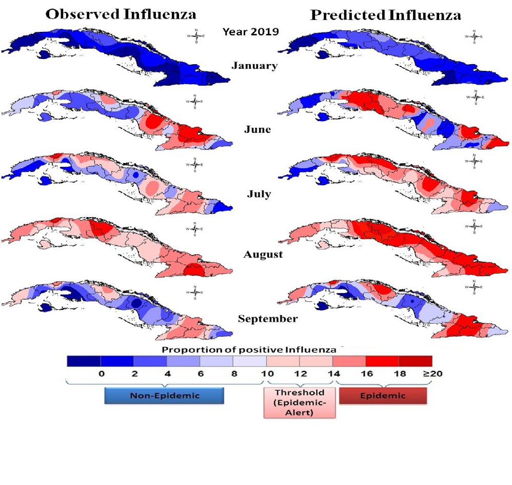
Once adjusted and reached a plausible and stable model to simulation of viral circulation comportment at spatial scale, some estimates were done for the month of higher viral circulation (June) and for the month of lower circulation (January), and to assess the quality of the results regarding the estimate and real behavior. The Skill factor (βi) for January 2016 was 0.9016 with a concordance index (Di) of 0.9112 meanwhile to June the Skill decreased to 0.8521 and the concordance to 0.8601. To both items a positive bias was sustained with values between 0.065 and 0.241 with ECM of 0,086 and 0.0277 respectively. Similar occurred in the same months of 2016 with low values of EMA between 0.076 and 0.405 respectively.
In Figure 3 the forecasted and real values of influenza virus circulation according to the seasonal climate prediction are presented, expected in the rainy period and in January corresponding to the dry period, for one of the proof years (2019), where a big great concordance is confirmed between the real and forecasted values, being June with the lower concordance.
Seasonal Forecast for Early Warning using the Spatial Model
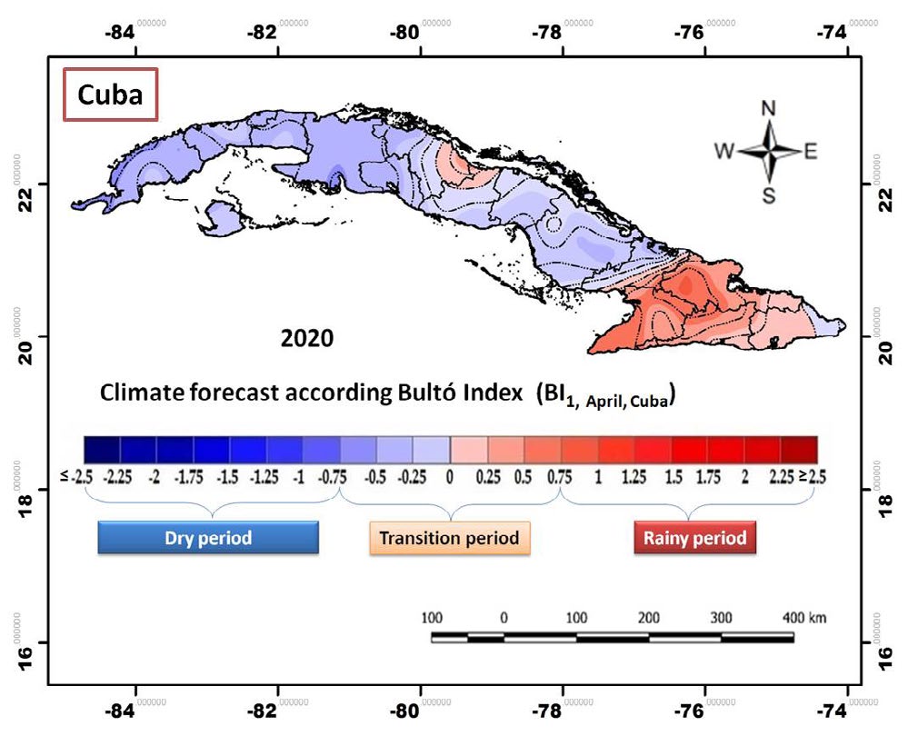
The spatial representation (Figure 4) of the expected climate behavior according to BI1,t,c index reflects the forecast of the climate variability signal for the first month of the temporal forecast in the quarter April-June.
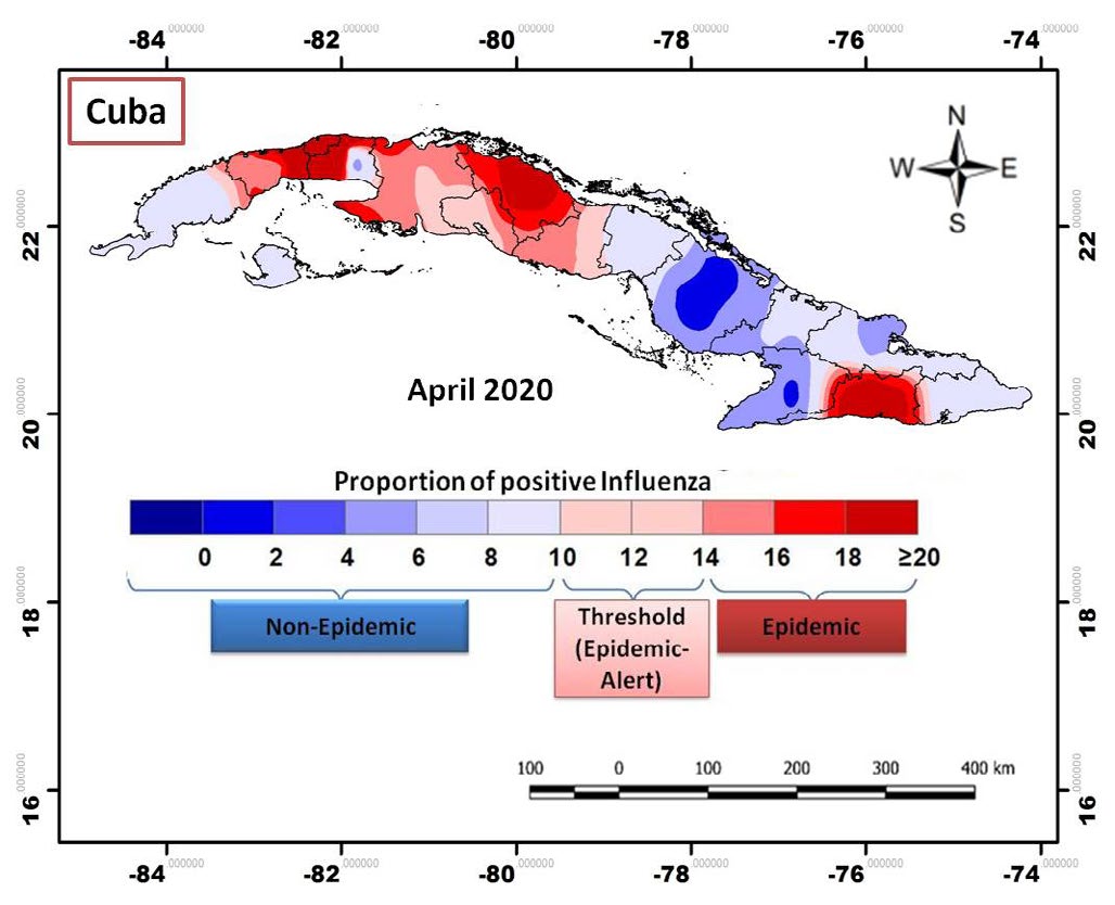
An example of forecast for the influenza risky areas according to the climate variations forecasted for April 2020 by BI1,April,Cuba climatic index is showed in Figure 5. A
month April less cold than the typical is expected, with some contrasts regarding the combined thermal regime with precipitations areas is important to highlight that values class predicted for the month are more proper for May than for April. Those conditions favor the increasing of influenza virus circulation in several geographic areas of the country. The forecast map of influenza virus circulation for the country indicates there are some regions at risk, as surpass the security threshold, and other regions advance toward such a situation. That is associated to the climatic conditions forecasted of high temperatures and humidity.
Discussion
Sensibility of Influenza Virus´s Behavior to Climate
The maximum values of influenza virus circulation are concentrated in the months May-September, belonging to the rainy season (May-October), when conditions are warmer and less contrasting, although not presented with the same intensity every year. This corresponds with a dynamic seasonal pattern. Even though there are two moments in the series with maximum values (2013 and 2015), in general a trend to decreasing towards 2018 are observed. It is also observed a clear inter-annual variation (alternating years of high circulation). Likewise, a clear inter-annual and seasonal variability is observed [18]. Those variations coincide with those described by other studies in the region where influenza circulates during rainy months (summer), but differ of the studies from temperate climate countries where circulation is during winter or in less rainy periods [18, 47].
Analysis of Temporal Model
With the temporal model, previsions could be done about the future evolution of epidemiological virus patterns up to three months in advance, starting from the last updated months in the model. The variables describing the climatic anomalies of BI1,t,c, hold a cumulative effect (lag or feedback) on the virus dynamic which last up to three months.
The proposed models are more plausible than those presented by other authors [20, 21, 44], because our models take into account the features of virus infections, which have marked variability and mean changes, as well as no- lineal autoregressive models with change in variance in an explicit form. Simulating the virus´s circulation and variation as described in the historical records, a bigger consistency of results is provided. It is also possible to predict picks and changes of volatility in the time. Another stronghold of these models is that allow simulating the influence of climate on the virus seasonal pattern, with a complex approach. Indexes describing climate variations which may alter the virus behavior and circulation are described, as the indexes perceive all changes of climate variations and the influence between them, and non from every variable separate [18].
So, the approach integrating all the climate variables allows understanding the better pattern of virus circulation and its associated phenomena. If there are high humidity and temperatures, it is generally a variable answer to a characterized climate situation that could be conditions by the presence of a low pressure system bringing convection processes [18, 48].
On the other hand, it is added that climate conditions, being more or less warm, affect blood circulation, cardiac rhythm and breathe in the human body, because the heat exchange is closely bound to the metabolic process, which is regulated by the nervous system. It can also debilitate the respiratory system interfering with the oxygen and carbon dioxide exchange, carrying a higher acidification of respiratory three, condition very favorable to the virus multiplication [49].
It means climate conditions of high humidity and temperature could favor the incubation of influenza viruses, while in other climatic situations could make the organism more resistant, which could facilitate or not the processes of condensation and acidification of airways. All these ease simulating the circulation of viruses by months and understanding what happens during the months July- August, which is the period when the human being in the study region receives the higher negative effect of climatic variations. Warmer and more humid conditions favor the viral circulation that, when conjugate with the contaminant burden (acting as irritants of airways), make increase the risk [18, 20].
Another strengthen of these models is that ARCH component is simulating the variability (volatility) of viral circulation produced in the previous month and recognizing the autoregressive component of the information, while the climatic variability in the ARCH component is simulating the influence on the variability of viral circulation pattern. That allows to incorporate the more updated signal of the series period where a change in the presence and intensity of the outbreak was presented, associated to an intervention, or a climate anomaly described by means of the climatic indexes before mentioned, about the behavior of influenza viruses.
For example, if the disturbance because of a rainy process appears with very warm conditions, as a consequence of anomalies in the global or regional circulation bringing a wide contrast. Using preceding models, the previous signal of variability, can be simulated given the monthly and bimonthly variation produced regularly, which remained expressed by the autoregressive component. Meanwhile, the change in the amplitude of the variability signal of a process to another, keeps collected in the change component of the variance, which is forecasted. They allow simulating the variability (volatility) of viruses, since the incorporation to climates by complex climatic indexes propitiating minor prediction errors, being considered independent the picks simulation [46]. In conclusion, the models found are adequate and give the possibility of being used for surveillance of climate hazard situations for human health.
Spatial Model
The values obtained from spatial model fitness evidence the specified model is correct, and represents the spatial characteristics and variations, so as virus as the climate influence on the spatial pattern and the classes obtained, matching with the criteria stated by Anselin for selection of autoregressive spatial model with exogenous variable (SARX) [29].
The model permits simulate the spatial relationship, which are modulated by endogenous effects (by the behavior pattern of the own series) and exogenous (climatic conditions, social, etc.). It means, it allows to describe the climatic conditions influencing in the virus circulation in the regions or areas A and how them influence in the region or areas B. Those aspects may explain the virus dispersion at spatial scale and in some way to understand its spatial dynamic. Besides, to determine the areas or regions of higher circulation and them an increasing of ARI cases associated to influenza virus.
It is possible to applicate this model to study the spatial- temporal distribution of another virus [18, 19]. So, this approach could be applied to the new coronavirus SARS-CoV-2 causing the Covid-19 that currently generates a pandemic with a high case fatality rate, from the considerations performed by Italian authors corroborating its usefulness [50, 51, 52]. Dynamics of SARS CoV-2 in our tropical climate has an important effect in the ARI High circulation in months of the rainy period of high temperatures and high humidity, coinciding with the picks of bigger intensity of the ARI in Cuba [47].
Quality of Temporal and Spatial Forecasts
Temporal
The proposed models were adequate for the prediction, because the prognosis errors were minimum. The experimental monthly forecast performed during the years 2017- 2019 match with what happened in the country. This evidences that the model keeps stable if comparing with the validation results with the independent sample of 2016. That overcame the predictive capacity and quality regarding the concordance described by other authors reported so far [21, 32].
Spatial
In the representation of the spatial predicting models for the months of rainy and less rainy periods, a clear spatial variation can be observed and the virus dynamic dispersion in the country, describing the increasing and decreasing of virus circulation, according to the different areas in the country. Those present adequate conditions for the viral circulation and are characterized by authors a bigger frequency of very humid days, with high frequency of cloudy days, high number of rainy days, low thermal contrast and decreasing of sunny days. Those variations remained described inside the model in a significant way by the index (BI1,t,c). These conditions are propitious for virus increasing and its multiplication, which have been exposed in previous studies from several authors [17, 18, 53, 54].
These results corroborate that complex indexes describing the climate variability are excellent predictors of the influenza virus spatial configuration [18, 17]. So, it is possible to perform virus forecasts, which agree with the studies of Wan Yang and Sophia associating climatic elements with the influenza dynamic in Africa and other tropical countries [53, 54].
The signs of all model coefficients are positive, which confirm that positive anomalies during rainy period (more humid and warmer), favor the virus circulation, contrary to that happening during the less rainy period. It is remarkable the high significant and quality of the fitness obtained. Besides, it is confirmed that the virus spatial distribution presents a spatial structure, which is hold to physic- geographic characteristics of the place, the climate variations and the own virus characteristics.
The virus forecast representation with prognostic maps allows predicting the circulation and dispersion of the virus activity on a friendly and very clear way¸ which may facilitate to decision-makers the interventions, since indicates the risky areas at provincial level with conditions to the appearance of an influenza epidemic. This result gives an answer to the need required by early warning systems for health and satisfies the recommendations performed by other authors [21].
The Seasonal Forecast and its Usefulness for the Early Warning
Temporal forecast evidences an increasing in the influenza virus circulation for the months April to June, being May the month when higher circulation is expected associated to climatic conditions forecasted (humidity, rainy, cloudy days and high temperatures). Furthermore¸ 2020 should be of high influenza activity, as a biannual epidemic cycle has been described [18].
Even is important the temporal seasonal forecast, it is also essential for early warning to identify the areas where highest risks are expected. The forecast map of BI1,t,Cuba shows the signal of climate variability for April, in which the highest values of climatic anomalies are framed in a very high intensity class (above 95 percentile) to eastern provinces and part of the central region with zones of alternation to low. Meanwhile, for western provinces the values are framed in the medium intensity class, as indicates the index stratification; it means, very hot and humid conditions.
The information presented in the early warning is very useful and allow the health authorities the beginning of an anticipated response and decision taking in high risk areas to reduce outbreaks and prevent epidemics. The early warning reduces the response time between detection of first’s cases and reaction of surveillance system to take actions, as stated by other authors [26, 28, 45]. The results also coincide with Chadsuthi [32] regarding its purpose and the use of climate though differs in the kind and order of the model and the way in which incorporates climate as an exogenous variable to explain the associations.
Scope and limitations of Models Proposed
Statistic models considering the variance change, position and spatial distribution in an explicit way, have yet limitations, although have had a wide development in the last decades, so in the advances in methods (i.e. asymmetry modelling), as by the geo-referenced data availability (virological and climatic) [32, 55, 56].
A limitation of the model is that being influenza data an aggregated information (taken from administrative- geographic areas: provinces, municipalities, etc.), sometimes could not be the most proper to describe the phenomenon on study. No necessarily are adjusted to the geographic unit. This work approach continuous being preferred, because represents the capacity of simulate in a joint manner the complex interactions between seasonal climatic variations, the susceptibility of human beings and virus, with the individual risk of getting sick with influenza, in both spatial and temporal scale [57]. Geographic conditions like altitude, longitude and latitude described in the spatial model may be incorporated, which remain being an advantaged approach and used to climate-health studies regarding the other models [57].
Conclusion
Based in the relationship and mechanisms between climatic variability and the behavior of influenza viruses, integrated models AR (p)-ARCHX (q) for the temporal scale and simultaneous autoregressive models (SARX) to the spatial scale are obtained, both with exogenous variables, which permits simulate and forecast with a high capacity, the circulation and spatial dynamic of influenza virus in the country beginning with the seasonal climate variation in Cuba.
The utility of seasonal prediction is evidenced according to Bultó indexes, with enough anticipation. Forecasting maps show the year period and country an area where climate impacts and favor the more favorable conditions for the beginning of outbreaks and viral circulation, with is a tool for early warning.
The methodology approach and models used to study the spatial dynamic and to perform the influenza virus prediction, could be applied to understand the distribution and spatial dynamic of the new coronavirus SARS CoV-2.
Conflict of Interests
The authors declare that there is no conflict of interests regarding the publication of this paper.
Acknowledgment
The Project “Impact of climate on Aedes aegypti, dengue, Acute Diarrheal Disease, Acute Respiratory Infections by RSV and Influenza in the context of another environmental, demographic, epidemiological and microbiological variables) was supported by the Ministry of Science, Technology and Environment (grant P211LH007–0023) and the Ministry of Public Health (grant 131089). Authors acknowledge to the personnel of the National Reference Laboratory for Influenza and other Respiratory Viruses at the Institute of Tropical Medicine ‘’Pedro Kourí’’ (IPK), Havana, Cuba, as well as to the personnel of the meteorology stations network at the Institute of Meteorology in de Cuba.
References
-
Arencibia A, Piñón A, Muné M, Acosta B, Valdés, et al. (2014) Molecular characterization of influenza A viruses circulating in Cuba between April 2009 and August 2010. J Infect Dev Ctries 8(7): 929-932.
-
Luengo GS (2017) Influenza viruses: genetic variation and pathogenesis. Universidad Complutense de Madrid.
-
Victoria YF, Dean TJ, Lawrence HS (2018) Pandemic risk: how large are the expected losses?. Bull World Health Organ 96: 129-134.
-
(2000) Programa Integral de Atención y Control de las IRA. Ministerio de Salud Pública República de Cuba.
-
Gregg MB, Hinman AR, Craven RB (1978) The Russian flu: Its history and implications for this year’s influenza season. JAMA 240(21): 2260-2263.
-
Bishop JF, Murnane MP, Owen R (2009) Australia’s winter with the 2009 pandemic influenza A (H1N1) virus. N Engl J Med 361(27): 2591-2594.
-
Shaman J, Pitzer VE, Viboud C, Grenfell BT, Lipsitch M (2010) Absolute humidity and the seasonal onset of influenza in the continental United States. PLoS Biol 8: e1000316.
-
Elert E (2013) FYI: Why Is There A Winter Flu Season?. Popular Science, pp: 324.
-
(2015) The Flu Season. Centers for Disease Control and Prevention.
-
Viboud C, Alonso WJ, Simonsen L (2006) Influenza in tropical regions. PLoS Med 3(4): e96.
-
Lipsitch M, Viboud C (2009) Influenza seasonality: lifting the fog. Proc Natl Acad Sci 379(106): 3645-3666.
-
Moura FE, Perdigao AC, Siqueira MM (2009) Seasonality of influenza in the tropics: a distinct pattern in northeastern Brazil. Am J Trop Med Hyg 81(1): 180-183.
-
Tamerius J, Nelson MI, Zhou SZ, Viboud C, Miller MA, et al. (2011) Global influenza seasonality: reconciling patterns across temperate and tropical regions. Environ Health Perspect 119(4): 439-445.
-
Shaman J, Goldstein E, Lipsitch M (2011) Absolute humidity and pandemic versus epidemic influenza. Am J Epidemiol 173(2): 127-135.
-
Tamerius JD, Shaman J, Alonso WJ, Bloom-Feshbach K, Uejio CK, et al. (2013) Environmental predictors of seasonal influenza epidemics across temperate and tropical climates. PLoS Pathog 9(3): e1003194.
-
Durand LO, Cheng PY, Palekar R, Clara W, Jara J, et al. (2016) Timing of influenza epidemics and vaccines in the American tropics, 2002–2008, 2011–2014. Influenza Other Respir Viruses 10(3): 170-175.
-
Acosta B, Piñón A, Arencibia A, Valdés O, Muné M, Savón C, et al. (2016) Contributions of the influenza laboratory surveillance for monitoring the effectiveness of the vaccination. Virol-mycol 5: 1.
-
Vega YL, Ortiz PLB, Acosta BH, Valdés OR, Borroto SG, et al. (2018) Influenza’s Response to Climatic Variability in the Tropical Climate: Case Study Cuba. Virol & Mycol 7: 1000179.
-
Ortiz-Bulto PL, Vega YL, Ramírez OV, Herrera BA, Gutiérrez SB (2017) Temporal-Spatial Model to Predict the Activity of Respiratory Syncytial Virus in Children Under 5 Years Old from Climatic Variability in Cuba. Int J Virol Infect Dis 2(1): 030-037.
-
Ray J, Brownstein J (2013) Forcasting influenza outbreaks using open-source media reports. SANDIA REPORT. SAND2013-0963. Prepared by Sandia National Laboratories Albuquerque, New Mexico 87185 and Livermore, California.
-
La Fuente ODM, Febrero-Bande M, Muñoz MP, Domínguez À (2018) Predicting seasonal influenza transmission using functional regression models with temporal dependence. PLoS ONE 13(4): e0194250.
-
Ortiz PL, Pérez A, Rivero A, Pérez AR, Canga R (2013) Human Health In: Planos E, et al. (Eds.), “Impacts of climate change and adaptation measures in Cuba”. Institute of Meteorology, Environment Agency, Ministry of Science, Environment and Technology Cuba, pp: 401- 430.
-
ONEI (2019) Cuban Statistical Yearbook 2018. Chapter 1: Territory, Cuba, pp: 15.
-
Ortiz PL, Guevara V, Díaz M, Pérez A (2000) Rapid assessment of methods /models and human health sector sensitivity to climate change in Cuba. Climate Change: Impacts and Responses, pp: 203-222.
-
Ortiz PL, Rivero A, Linares Y, Pérez A, Vázquez JR (2015) Spatial models for prediction and early warning of Aedes aegypti proliferation from data on climate change and variability in Cuba. MEDICC Rev 17(2): 20-28.
-
Hirve S, Newman LP, Paget J, Azziz-Baumgartner E, Fitzner J, et al. (2016) Influenza Seasonality in the Tropics and Subtropics When to Vaccinate?. PLoS ONE 11(4): e0153003.
-
Beckett CG, Kosasih H, Ma’roef C, Listiyaningsih E, Elyazar IR, et al. (2004) Influenza surveillance in Indonesia: 1999-2003. Clin Infect Dis 39(4): 443-449.
-
Luc Anselin SJR (2014) Modern Spatial Econometrics in practice. A Guide to GeoDa, GeoDaSpace and PySAL, Chicago, pp: 354.
-
Loomis JM, Da Silva JA, Philbeck JW, Fukusima SS (1996) Visual perception of location and distance. Current Directions in Psychological Science 5(3): 72-77.
-
Gaetan C, Guyon X (2010) Spatial Statistics and Modeling. Springer Science, pp: 307.
-
Ortiz Bultó P, Pérez Rodríguez AE, Rivero Valencia A, Pérez Carrera A, Vásquez Cangas JR, et al. (2010) Impacts of climate variability and change on the health sector in Cuba. Meteorología Colombiana 40: 79-91.
-
Chadsuthi S, Iamsirithaworn S, Triampo W, Modchang C (2015) Modeling Seasonal Influenza Transmission and Its Association with Climate Factors in Thailand Using Time-Series and ARIMAX Analyses. Comput Math Methods Med 436495.
-
Engle RF (1982) Autoregressive Conditional Heteroscedasticity with Estimates of the Variance of the U.K. Inflation Econometrical 50(4): 987-1008.
-
White H (1980) Heteroscedasticity-Consistent Covariance Matrix Estimator and a Direct Test for Heteroscedasticity. Econometric 48(4): 817-838.
-
Breusch TS, Pagan AR (1979) A Simple Test of Heteroscedasticity and Random Coefficient Variation. Econometric 47(5): 1287-1294.
-
Stavros D, Evdokia X (2004) Autoregressive Conditional Heteroscedasticity (ARCH) Models: A Review. Quality Technology and Quantitative Management 1(2): 271- 324.
-
Fernández CMA (2003) Heterocedasticidad Condicional, Atípicos y Cambios de Nivel en Series Temporales Financieras. Universidad Carlos III De Madrid, pp: 1-188.
-
Wiliam WS (1990) Time Series Analysis (Univariate and Multivariate Methods). New York: Addison Wesley. USA
-
Chasco CY (2003) Spatial econometrics applied to the prediction-extrapolation of micro-territorial data. Dialnet.
-
Chow A, Ma S, Ling AE, Chew SK (2006) Influenza- associated deaths in tropical Singapore. Emerg Infect Dis 12(1): 114-121.
-
Nguyen HL, Saito R, Ngiem HK, Nishikawa M, Shobugawa Y (2007) Epidemiology of influenza in Hanoi, Vietnam, from 2001 to 2003. J Infect 55(1): 58-63.
-
Moura FE (2010) Influenza in the tropics. Curr Opin Infect Dis 23(5): 415-420.
-
Ramos PA, Fernández OS, López AC, Galindo B, Herrera AB, et al. (2005) Influenza and vaccination. Rev Biomed 16: 45-53.
-
Moreno RS, Vaya EV (2000) écnicas econométricas para el tratamiento de datos espaciales: La econometría espacial. Edición de la Universidad de Barcelona, pp: 158.
-
Coelho CA, Barbara B, Laurie W, Marion M, Barbara Cl (2019) Chapter 16 - Forecast Verification for S2S Timescales. Sub-Seasonal to Seasonal Prediction 337- 361.
-
Wilks D (2011) Statistical methods in the atmospheric sciences. 3rd (Edn.).
-
Borroto S, Linares Y, Ortiz P, Valdés O, Acosta B (2020) Influence of climatic variability and respiratory viruses on the burden of medically attended acute respiratory infections in Cuba. J Respir Dis Med 2: 1-7.
-
Lecha LB, Paz LR, Lapinel B (1994) The Climate of Cuba. Editorial Academia, La Habana, Cuba, pp: 186.
-
Ishmatov A (2017) On the connection between supersaturation in the upper airways and «humid-rainy» and «cold-dry» seasonal patterns of influenza. Peer J Pre Prints, pp: 1-14.
-
Paul M, Held L (2011) Predictive assessment of a non- linear random effects model for multivariate time series of infectious disease counts. Statistics in Medicine 30(10): 1118-1136.
-
Giuliani D, Dickson M, Espa G, Santi F (2020) Modelling and predicting the spatio-temporal spread of Coronavirus disease 2019 (COVIC-19) in Italy. BMC Infectious Diseases.
-
Passerini G, Mancinelli E, Morichetti M, Virgili S, Rizza U (2020) A Preliminary Investigation on the Statistical Correlations between SARS-CoV-2 Spread and Local Meteorology. Int J Environ Res Public Health 17(11): 4051.
-
Yang W, Cummings MJ, Bakamutumaho B, Kayiwa J, Owor N, et al. (2018) Dynamics of influenza in tropical Africa: Temperature, humidity and co-circulating (sub) types. Influenza and Other Respiratory Viruses 12(4): 446-456.
-
Sophia NG, Gordon A (2015) Influenza Burden and Transmission in the Tropics. Curr Epidemiol Rep 2(2): 89-100.
-
Tong H (1990) Non-linear time series: A dynamical system approach. Oxford University Press.
-
Messner SF, Anselin L (2002) Spatial analysis of homicide with areal data, pp: 1-37.
-
Tompkins AM, Lowe R, Nissan H, Martiny N, Roucou P (2019) Chapter 22-Predicting Climate Impacts on Health at Sub-seasonal to Seasonal Timescales. Sub-seasonal to Seasonal Prediction, pp: 455-477.
- Diversity of Candida sp and Antifungal Susceptibility Patterns in Digestive Candidiasis among People Living with HIV in CHU of Libreville, Gabon
- Vulvovaginal candidiasis: Retrospective study (2019- 2021) at the Centre Hospitalier National de Pikine, Suburban Dakar, Senegal
- Identification of Environmental Fungal Species in Clinical Services of University Hospital of Angre, Abidjan (Cote d’Ivoire)
- New Location of some Gasteroid Basidiomycetes in Western Kazakhstan
- Evaluation of Various Extracellular Enzymes of Ectomycorrhizal Mushrooms
- Morphology and Phylogeny of Lactarius Wallichianae sp. nov and Xerula magnispora sp. nov. from India