Sensitivity Tests of Parameters in Laboratory Polymer Flood Analysis
The results of preliminary polymer flood laboratory study, including the matched coreflood simulation model results were shown to decide about analytical procedure for more detailed polymer flood study. The coreflood model is confirmed as feasible by comparing the recovery after waterflood period and after the polymer flood period. Sensitivity analysis of fluid compressibilities, parameters that affect polymer solution rheology, relative permeability and polymer adsorption index was perfumed both in laboratory and by simulation model. The results shown how different parameters affect recovery and additional recovery from polymer flood versus time. This method helped to speed up the assessment of critical parameters which should be measured and analyzed in more detailed study.
Introduction
The viscoelastic properties of polymers are making them attractive medium for improving the waterflood oil recovery. When considerable pore volume is saturated with oil left behind in the reservoir after classic waterflood, polymer may be effective in decreasing the mobility of brine by mixing and consequently decreasing brine-oil mobility ratio. The decrease of mobility ratio is desirable because injected brine velocity and thus the viscous fingering of brine will be reduced. Viscous fingering is the phenomenon that occurs when displacing fluid is less viscous than oil. This effect is pronounced in heterogeneous reservoirs, with oil viscosities higher than 10 mPas. Oil viscosity criteria is dependent on oil price and polymer price (which is falling below $4/kg). Polymer quality is determined by its rheological properties and by its stability which is affected by shear forces, injection speed, thermal degradation and interaction with other fluids, primarily with brine of some salinity and chemical composition. The laboratory studies of viscous fingering during a waterflood may be unreliable which is assigned to scaling issues i.e. to small diameter and the length of core samples. This makes coreflood simulation a good method to build a predictive model that can be used for further reservoir simulations and field development.
This paper will present the steps from the establishment of laboratory workflow (measurements) for polymer flood to full laboratory study accompanied by measured data interpretation, coreflood study and polymer flood design. Detling proposed using water-soluble polymers in order to increase the viscosity of water [1]. Sandiford reported the results of their laboratory and field studies, concluding that oil recovery will be achieved due to improvement in sweep efficiency, microscopic displacement efficiency and combination of these mechanisms [2]. They used sand packs (10 cm to 12 m) for their analysis of displacement in linear system, achieving up to 100 % sweep efficiency which they attributed to homogeneity and anisotropy of the system which will primarily reflect microscopic displacement.
Jewett and Schurz published an overview of success for 61 polymer flooding projects and characterized them as:
- Successful projects (a - projects that are completed, and data about economics were published, b – projects that expanded from pilot to commercial, c - commercial projects which performance to date was encouraging)
- Unsuccessful projects (no expansion of a project or recovery reported)
- Unsuitable projects (a - reservoirs with sizeable gas- cap, b - reservoirs with large influence of an aquifer, c - wells with severe injectivity problems, d - fractured zones or thief zones with high permeability)
- Recently initiated projects.
Such analysis resulted with the tables of parameters values that are common for successful projects Table 1.
| min | max | |
|---|---|---|
| Mobility ratio, M | 0.1 | 42 |
| oil viscosity, (mPas) | 0.07 | 126 |
| Dykstra-Parsons heterogeneity coefficient (permeability variation, VDP) | 0.28 | 0.8 |
| Mobile oil saturation, So-Sor | 0.15 | 0.46 |
| Initial water saturation, Swi | 0.1 | 0.47 |
| Slug size, part of pore volume (PV) | 0.07 | 0.33 |
| permeability, k (mD) | 20 | 2300 |
| depth, h (m) | 121 | 1981 |
| temperature, T (°C) | 21 | 110 |
Table 1: Values of key parameters for successful polymer flooding projects (after data in Jewett and Schurz) Table 1: Values of k
Table 1: Values of key parameters for successful polymer flooding projects (after data in Jewett and Schurz) Table 1: Values of key parameters for successful polymer flooding projects (after data in Jewett and Schurz) Chauveteau and Kohler tested the performance of polymer solutions using partially hydrolyzed polyacrylamide and a polysaccharide, focusing on the analysis of stability conditions of solutions over long periods of time, including the effects of additives used during the injection, such as antioxidants and bactericides [3]. For flow properties, they performed low-speed injections of various solutions through short and long sandpacks. They detected the increase of polymer retention at high flow rates, and proposed performing experiments at several rates that are expected during waterflood in a reservoir. Retention occurs due to adsorption in an irreversible manner and due to trapping in no-flow areas. Szabo analyzed stratified and single layer systems, injected polymer slug sizes (pore volumes, PV) and various concentrations of a polymer [4]. He proved that the amounts of retained polymer (and improvement in oil recovery) are greater in stratified systems.
Castagno described their methodology for evaluation, based on real reservoir proposed for polymer flood [5]. They used fractional flow analysis with relative permeability from clean-core experiments and different viscosities of polymer solution. The analysis included reservoir characteristics, comparison of polymers, injectivity tests both on cleaned core samples and in well at the field, polymer stability, viscosity study and field evaluation for different polymer solutions. They reported bacterial control issues by means of severe near-wellbore degradation after 2-week shut-in period, as opposite to laboratory results. Primarily for this reason and the low effective viscosity of the polymer solutions, the proposed polymer flood project was denied. Wang gave an interesting review about Daqing oil field, where more than 1000 wells are polymer flooded [6, 7, 8]. They reported about 10-12% of additional oil recovery after waterflooding, and the decrease of water cut from
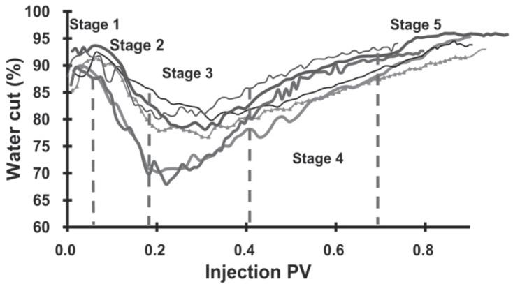
90% to 70%.More than 106 m3 of polymer solution has been injected to Daqing oil field. They described how the elasticity of a polymer affects displacement efficiency and the proposed use of low salinity water, high-molecular polymers, the use of higher polymer concentrations (to achieve increase of the elastic modulus for a polymer mixture). They investigated at pilot wells and based on simulation model as well, polymer flooding dependence on permeability layering and concluded that separate layer injection should be implemented. They detected five stages of polymer flooding Figure 1:
- initial stage (up to 0.05 PV polymer-solution injected) – the effects of polymer flood is not notable
- the response stage (0.05 to 0.2 PV polymer-solution injected) – polymer starts to improve oilrecovery, oil bank is formed and up to 15% of additionally recovered oil is produced
- stable water cut (0.2 to 0.4 PV polymer solution injected) – 40% of total additional recovery is recovered in that period, and produced polymer concentration increases
- increasing water cut (0.4 to 0.7 PV) – oil production decreases, areal sweep is at its maximum, about 30% of total additionally recovered oil is produced in that period
- Follow-up water drivestage (from the end of polymer injection to water cut about 98%) – produced polymer rate decreases, water cut increases, and total produced fluid slightly increases.
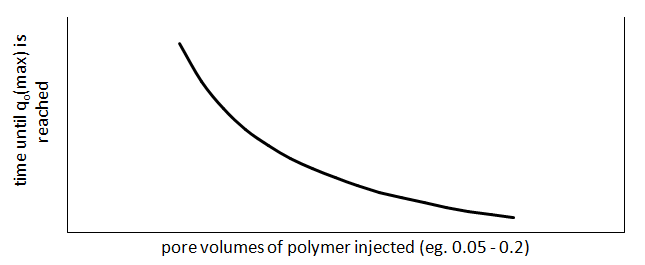
Based on experience, lab and literature data, we found the power-law relationship between polymer flooding injection rates and time to maximum oil production rate Figure 2. This parameter helps in economic analysis of a polymer flood project. Because the injection rate is inversely proportional to additional recovery, it should be balanced with target additional recovery i.e. profit from polymer flood project.
- Polymer-solution viscosity, which increases sweep efficiency
- Polymer molecular weight, which improves the polymer-solution viscosity, but also can decrease injectivity
- Polymer-solution concentration, which affects water cut, injectivity and the size polymer solution slugs.
- Polymer stability, which depends on polymer frontal advance velocity and interaction with other fluids
- Injectivity and injection rate – injectivity and pumping energy are directly connected with economics of polymer flood project.
On the other side, high injection rate can cause flow out of the pattern (target zones). Because chemical flood is sensitive to volatility of oil market, and despite the improvements and new discoveries in related technologies, since 1990 the most chemical and polymer flood has been performed when sustainable field development strategy is applied [9, 10, 11, 12, 13]. Such sustainable oil field development is typical for China. However, polymer flooding technology is improving and it is used in many countries: Carmopolis, Buracica and Conto de Amaro in Brasil, Sandand in India, Marmul in Oman [14], Pirawath in Austria, El Tordillo in Argentina, Horsefly Lake in Canada, Bochstedt in Germany, North Burbank and Pelican Lake are just some of examples in USA [14, 15]. In more than 90 % polymer floods HPAM type of polymer is used then PAM [16, 17, 18, 19]. Polysaccharides(Xantham and Schizophyllan i.e.
biopolymers) are intensively investigated in the case of high brine salinity and high reservoir temperatures [20].
Experimental and Simulation Procedure
Experiments
The study has been performed for an oil field in Drava depression, Croatia, starting with PVT analysis of oil, reservoir brine analysis and routine core analysis. Capillary pressures were measured with porous plate, centrifuge and Purcell’s method for a number of samples and by porous plate method for a sample used in for polymer flood. Reservoir brine of 20 g/L salinity was prepared to saturate core sample to Sw= 100%.Brine for injection was prepared based on reservoir brine analysis Table 2. HPAM was a polymer used to prepare polymer solution. Prepared concentration was 1500 ppm. The rheological properties of prepared solution were investigated using Anton Paar MC 92 viscometer.
| Component | TDS, % |
|---|---|
| NaCl | 89,8 |
| NaHCO3 | 4,0 |
| KCl | 1,5 |
| MgCl2 x 6H2O | 1,0 |
| CaCl2 x 6H2O | 3,7 |
Table 2: Synthetic brine composition.
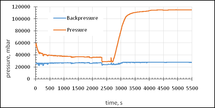
Table 2: Synthetic brine composition. Core was placed into triaxial core-holder and overburden pressure was applied and all measurements were performed at room temperature. Back-pressure was installed on the outlet of the core to maintain constant outlet pressure on a certain value. Effective permeability to water was determined in the next step. Afterwards, water displacement by oil was conducted in order to reach the value of Swi in the experimental core. By utilizing pressure transducers, it was possible to determine pressure stabilization across the core and announce end of the displacing process. Permeability to oil at Swi was determined. Brine was injected at the constant rate of 200 mL/h. The volume of oil displaced out of the core was collected into acoustic separator which determines the interface between oil and water and directly calculates displaced oil (water) volume. After the pressure was stabilized across the core sample (9 PV of water injected), flow was switched from water pump to polymer pump which injected 5 PV of polymer in the core at the rate of 100 mL/h. After final pressure stabilization with polymer injection, flow was switched again to water pump in order to determine the residual resistance factor (Rrf) which represents the value of permeability reduction to water which was caused by polymer retention on the pore walls.
Coreflood Simulation Model
Coreflood model was done in Schlumberger Eclipse, by using POLYMER option and parameters. We defined 5x25x25 grid, and tuned all the data that hadn’t been measured in the lab yet (polymer adsorption, Todd- Longstaff mixing parameters fluid and rock compressibilities, dead pore space, residual resistance factor etc.) [21]. The model doesn’t include any heterogeneity, and helps to assess the critical parameters for further laboratory analysis.
Experimental Data
Rheology
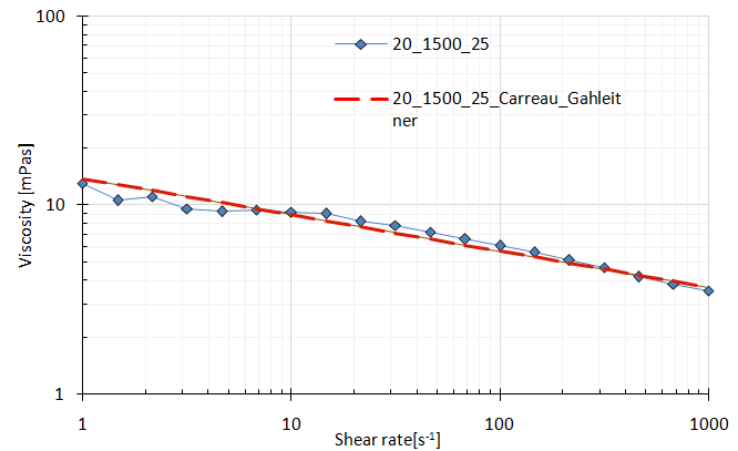
Polymer solution rheology was investigated by changing few key parameters which may affect polymer solution during flow under reservoir conditions. Therefore, salinity, temperature, polymer concentration in the solution and shear rate were studied in detail. Results which are given in Figure 3 and Figure 4 prove shear thinning behavior of polymer solutions, i.e. reduction in solution viscosity with increasing shear rate for 1500 ppm solution under 25°C. Experimental viscosity was plotted on log-logscale together with two regression models: Carreau–Gahleitner and Carreau-Yasuda which prove good fit [22, 23].
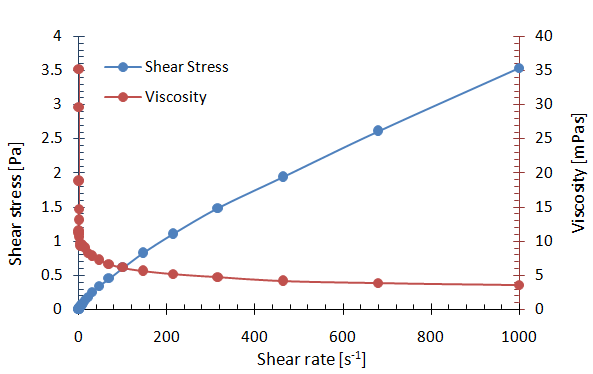
Sensitivity analysis was conducted for several parameters that affect polymer solution viscosity. For a base case in this example, salinity was 20 g/L, polymer concentration 1500 ppm and temperature 55°C. Deviation from the base case of any of parameters yields change in viscosity. Figure 5 depicts grey, orange, yellow and blue curves which represent concentration, salinity, shear rate and temperature, respectively.
Several polymer concentrations proved to be adequate to achieve the favorable mobility ratio (M) and the most economically feasible option was chosen to be applied for a further laboratory study, which was 1500 ppm concentration.
Coreflood Experiment
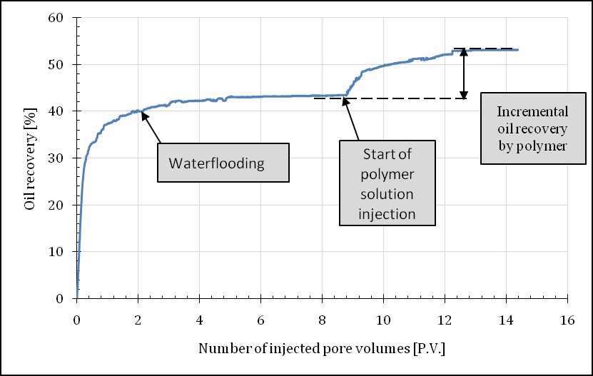
Coreflood oil displacement experiment was conducted in two stages. First stage involves waterflooding under constant injection rate, while the second stage involves polymer injection under 50% smaller, but also constant, injection rate. Details on pressure behavior during the experiment are shown in Figure 6 and Figure 7 shows the results of polymer flood.
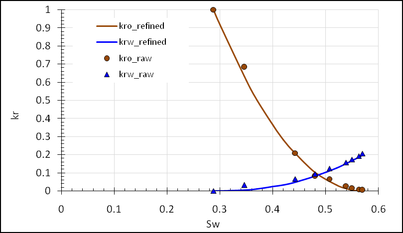
![Figure 6: Pressure curve during water and polymer injection. Having coreflood data available Figure 7, it was possible to construct relative permeability tables for a given system. For both components – brine model and polymer solution, single relative permeability (kr) table was calculated. After the construction of raw curves from laboratory measurements, it was possible to refine them by applying Corey exponents for oil and water (No and Nw) which were determined separately [24]. Relative permeability curves, both raw and refined, are given in Figure 8.](/fulltextimages/875/fig_6.png)
Figure 6: Pressure curve during water and polymer injection. Having coreflood data available Figure 7, it was possible to construct relative permeability tables for a given system. For both components – brine model and polymer solution, single relative permeability (kr) table was calculated. After the construction of raw curves from laboratory measurements, it was possible to refine them by applying Corey exponents for oil and water (No and Nw) which were determined separately [24]. Relative permeability curves, both raw and refined, are given in Figure 8.
Results and Discussion
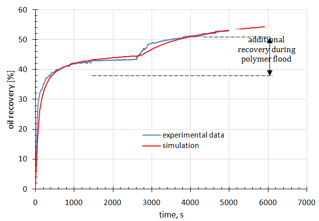
The shape of simulated oil recovery curve was in a good accordance with measured data we modified. Waterflood part gave somewhat more optimistic simulation results i.e. oil recovery was increasing at the end of waterflood. The same happened with polymer flood curve from simulation Figure 9.
- oil, brine and polymer compressibility
- more detailed polymer solution rheology analysis, because during reservoir simulation viscosities are needed at different shear rates, but also at different concentrations
- permeability and porosity heterogeneity study
4. relative permeability near critical saturations 5. adsorption index 6. capillary pressure These parameters were found as critical during simulation model tuning, and, after changing them, coreflood model showed good total recovery results Table 3:
| Recovery | d | Total Oil Recovered% | R | Aditional | ) | ||||
|---|---|---|---|---|---|---|---|---|---|
| After | ecovery (AR | ||||||||
| Waterfloo | After | ||||||||
| Period% | Waterflood% | ||||||||
| e | xperimenta | l | 43.55% | 53.16% | 9.60% | ||||
| simulation | 44.60% | 54.36% | 9.80% |
Table 3: Simulation and experimental coreflood results.
Conclusions
The results of preliminary polymer flood laboratory study were shown, including the analytical interpretation and testing of correlations. Coreflood simulation model was used to save time and decide about the whole procedure for a detailed polymer flood study, and to detect the parameters that affect the results of polymer flood and simulation model. Compressibility coefficients may help to adjust total cumulative productions. Adsorption parameters for polymer-rock system affect polymer additional recovery (AR). For a higher adsorption, AR in our model was lower. Capillary pressures (Pc), despite often being neglected in simulation studies, appeared as an important parameter. This is related to dead zones in polymer flood space, and it is hard to determine representative Pc table for a reservoir because of heterogeneity in porous structure. Relative permeability affects the shape of production curve. In our study, coreflood experiment was conducted at high velocities and details about relative permeability near critical saturations are not known. Single relative permeability curve (both for waterflood and then for polymer flood) can be used only for projects where no waterflood will occur after polymer flood, but it is suitable for analysis shown in this paper. This paper has shown that a method for a rapid polymer flood can be developed by using coreflood simulation model. This can significantly save time for extensive analyses that include time demanding wettability, capillary pressure and coreflood experiments.
References
-
Detling KD, Shell Dev (1944) Process of recovering oil from oil sands. U.S. Patent 2,341,500.
-
Sandiford BB (1964) Laboratory and field studies of water floods using polymer solutions to increase oil recoveries. Journal of Petroleum Technology 16(08): 917-922.
-
Chauveteau G, Kohler N (1974) Polymer flooding: The essential elements for laboratory evaluation. Society of Petroleum Engineers, SPE Improved Oil Recovery Symposium, ulsa, Oklahoma.
-
Szabo MT (1975) Laboratory investigations of factors influencing polymer flood performance. Society of Petroleum Engineers Journal 15(04): 338-346.
-
Castagno RE, Shupe RD, Gregory MD (1987) Method for laboratory and field evaluation of a proposed polymer flood. Society of Petroleum Engineers, SPE Reservoir Engineering 2(04): 452-460.
-
Wang D, Cheng J, Yang Q, Wenchao G, Qun L, et al. (2000) Viscous-elastic polymer can increase microscale displacement efficiency in cores. Society of Petroleum Engineers, SPE annual technical conference and exhibition, Dallas, Texas.
-
Wang D, Seright RS, Shao Z, Wang J (2007) Key Aspects of Project Design for Polymer Flooding. Society of Petroleum Engineers, SPE Annual Technical Conference and Exhibition, Anaheim, California, USA.
-
Wang D, Seright RS, Shao Z, Wang J (2008) Key aspects of project design for polymer flooding at the Daqing Oilfield. Society of Petroleum Engineers, SPE Reservoir Evaluation & Engineering 11(06): 1117- 1124.
-
Chang HL, Zhang ZQ, Wang QM, Xu ZS, Guo ZD, et al. (2006) Advances in polymer flooding and alkaline/surfactant/polymer processes as developed and applied in the People's Republic of China. Journal of petroleum technology 58(02): 84-89.
-
Delamaide E, Corlay P, Demin W (1994) Daqing oil field: The success of two pilots initiates first extension of polymer injection in a giant oil field. Society of Petroleum Engineers, SPE/DOE Improved Oil Recovery Symposium, Tulsa, Oklahoma.
-
Han DK, Yang CZ, Zhang ZQ, Lou ZH, Chang YI (1999) Recent development of enhanced oil recovery in China. Journal of Petroleum Science and Engineering 22(1): 181-188.
-
Li D, Shi MY, Wang D, Li Z (2009) Chromatographic separation of chemicals in alkaline surfactant polymer flooding in reservoir rocks in the Daqing oil field. Society of Petroleum Engineers, SPE International Symposium on Oilfield Chemistry, The Woodlands, Texas.
-
Wang D, Cheng J, Wu J, Wang G (2002) Experiences learned after production of more than 300 million barrels of oil by polymer flooding in Daqing oil field. Society of Petroleum Engineers, SPE Annual Technical Conference and Exhibition, San Antonio, Texas.
-
Moritis G (2010) Report on EOR/Heavy Oil: CO2 miscible, steam dominate enhanced oil recovery processes. Oil & Gas Journal.
-
Leonhardt B, Visser F, Lessner E, Wenzke B, Schmidt J (2011) From flask to field–The long road to development of a new polymer. IOR 2011-16th European Symposium on Improved Oil Recovery.
-
Zhijian Q, Yigen Z, Xiansong Z, Jialin D (1998) A successful ASP flooding pilot in Gudong oil field. SPE/DOE Improved Oil Recovery Symposium, Tulsa, Oklahoma.
-
Pu H (2009) An update and perspective on field-scale chemical floods in Daqing oilfield, China. Society of Petroleum Engineers_,_ Middle East Oil and Gas Show and Conference, Manama, Bahrain.
-
Pitts MJ, Dowling P, Wyatt K, Surkalo H, Adams KC (2006) Alkaline-surfactant-polymer flood of the Tanner Field. Society of Petroleum Engineers, SPE/DOE Symposium on Improved Oil Recovery, Tulsa, Oklahoma, USA.
-
Vargo J, Turner J, Bob V, Pitts MJ, Wyatt K, et al. (2000) Alkaline-surfactant-polymer flooding of the Cambridge Minnelusa field. Society of Petroleum Engineers, SPE Reservoir Evaluation & Engineering 3(06): 552-558.
-
Leonhardt B, Ernst B, Reimann S, Steigerwald A, Lehr F (2014) Field testing the polysaccharide schizophyllan: results of the first year. Society of Petroleum Engineers, SPE Improved Oil Recovery Symposium, Tulsa, Oklahoma, USA.
-
Todd MR, Longstaff WJ (1972) The development, testing, and application of a numerical simulator for predicting miscible flood performance. Journal of Petroleum Technology 24(07): 874-882.
-
Carreau PJ, Kee DD, Daroux M (1979) An analysis of the viscous behaviour of polymeric solutions. The Canadian Journal of Chemical Engineering 57(2): 135- 140.
-
Mezger TG (2006) The rheology handbook: for users of rotational and oscillatory rheometers. In: Rev. (Edn.) 3rd Vincentz Network, Hanover, Germany.
-
Brooks RH, Core AT (1964) Hydraulic properties of porous media. Hydrology Papers 3, Colorado State University, Fort Collins, Colo, pp: 27.
-
Batias J, Hamon G, Lalanne B, Romero C (2009) Field and laboratory bservations of Remaining oil saturations in a light oil reservoir flooded by a low salinity aquifer. Paper SCA2009-01 presented at the 23rd international symposium of the society of core analysts, Noordwijk aan Zee, The Netherlands, pp: 1- 12.
-
Mogollon JL, Lokhandwala T (2013) Rejuvenating Viscous Oil Reservoirs by Polymer Injection: Lessons Learned in the Field. Society of Petroleum Engineers, SPE Enhanced Oil Recovery Conference, Kuala Lumpur, Malaysia.
-
Olajire AA (2014) Review of ASP EOR (alkaline surfactant polymer enhanced oil recovery) technology in the petroleum industry: Prospects and challenges. Energy 77(c): 963-982.
- Nigeria’s Vulnerability in the Face of Global Energy Policy
- A Simulation Study of Investigation of Optimum Oil Production Performance by Applying Various Gas Injection Methods in Oil Reservoir
- Characterization of Permo-Triassic Reservoirs through Thermal Maturity Assessment of Westphalian Source Rocks in the Cheshire Basin
- Influence of Microwax on the Rheological and Thermal Behaviour of a Wax Crude Oil
- Real-Time Monitoring and Performance Optimization of Steam Injection in Heavy Oil Reservoirs Using Fiber Optic Sensing and Integrated Predictive Simulation Models
- Rapid On-Site Determination of the Total Petroleum Hydrocarbon Content of Soils by Handheld Fourier Transform Near-Infrared Spectroscopy: Development of a Global, Site- and Scanner- Independent Calibration Model