Prediction of the Rise velocity of Taylor Bubble in Vertical Tube
A single gas bubble moving under the influence of gravitational, inertial, viscous and interfacial forces, relative to another fluid contained in a vertical cylindrical tube. Two-phase flows through millimeter channels may exhibit different behaviors due to the surface tension becomes significant in small - size channels. Wall effect is important for millimeter channel. As the diameter of the circular tubes became small, the upward motion of the gas bubble is slowed down, and ceases completely when the tube size was sufficiently reduced (diameter less than 5 millimeter for air - water). The sphericity of the bubble cap was enlarged about 40% due to change of the tube diameter from 6 mm to 9.5 mm. Predicted Froude number was also increased by 0.04 to 0.2 for the enhancement of tube diameter from 6 mm to 9.5 mm. Fluidsurface interaction can become dominated in small-channel. So we are interested to investigate the bubble dynamics in millimeter channel.
Introduction
Shape of the nose of a Taylor bubble propagating through a stationary liquid column highly influences its rise velocity [1]. Bubble rises faster with more pointed nose where blunted nose retards the rate of propagation of the bubble [2, 3, 4, 5, 6]. In fact, the rise velocity of a Taylor bubble is an implicit function of its shape and any theoretical analysis attempting to predict the rise velocity should also take the bubble shape into cognition [7, 8, 9, 10]. Considering the complex hydrodynamics associated with Growing interest on gas-liquid two-phase flow in various process industry and petrochemical industries is the driving force of the present study. Hydrodynamics of gas Taylor bubble in different diameter pipes have been investigated in the present study. Over the years, the hydrodynamics of Taylor bubbles has attracted the attention of a number of researchers. In their pioneering works Dumitrescu [5] and Davies and Taylor 7 theoretically analysed the motion of elongated gas bubbles rising through a vertical tube filled with an ideal fluid. Dumitrescu [5] considered invisid flow of liquid approaching the stationary bubble at its rise velocity and obtained the potential function for flow of liquid in circular tubes. He has reduced the problem to determining the shape of the cavity and the velocity of rise under invisid flow conditions. He further assumed spherical nose of the bubble and plug flow in the falling liquid film and solved simultaneously for flow around the nose and the asymmetric film flow to obtain the bubble velocity and the frontal radius of curvature. Davies and Taylor concluded the bubble profile to be spherical at the top and flat below by a series of measurements of the film thickness of the liquid film in several photographs of single bubble rising through tanks containing nitrobenzene. They obtained the rise velocity of such bubble from theoretically both the measurement of pressure distribution over the surface of a solid of nearly the same shape as the bubble as well as for a sphere moving in a frictionless liquid. They reported better agreement of the inviscid flow analysis with experimental results.
**Experimental Procedure**
The air bubble rises by downward displacement of water. Such bubble can be observed during drainage of water from narrow tube and during gas-liquid slug flow. The bubble rise velocity was determined by a digital camera (SONY DSC-F717) and one movie breaker software (Total Video Converter) which divides video into frames per sec. Each experiment has been repeated for at least 5 times.
**Analysis**
Geometry of the nose of a Taylor bubble is shown in Figure 2, the nose is bullet shaped. To consider the relative motion of the bubble it is assumed that liquid approaches from infinity at a velocity $-\Upsilon$ (equal to the bubble velocity) and the bubble is stationary [10, 11, 12]. The origin of the coordinate system is taken at the stagnation points. According to the Joseph, the surface of the cap is given by $z = -h(r, \theta) = -(R - r(\theta)\cos \theta)$. Where $r(\theta) = R(1 + s\theta^2)$ and $s = \frac{r^2(0)}{D}$ is the deviation of the free surface from perfect sphericity. $D$ is the tube diameter. Near the stagnation point $\theta = 0$ and $r(\theta) = R$ which is constant and bubble is perfectly spherical.
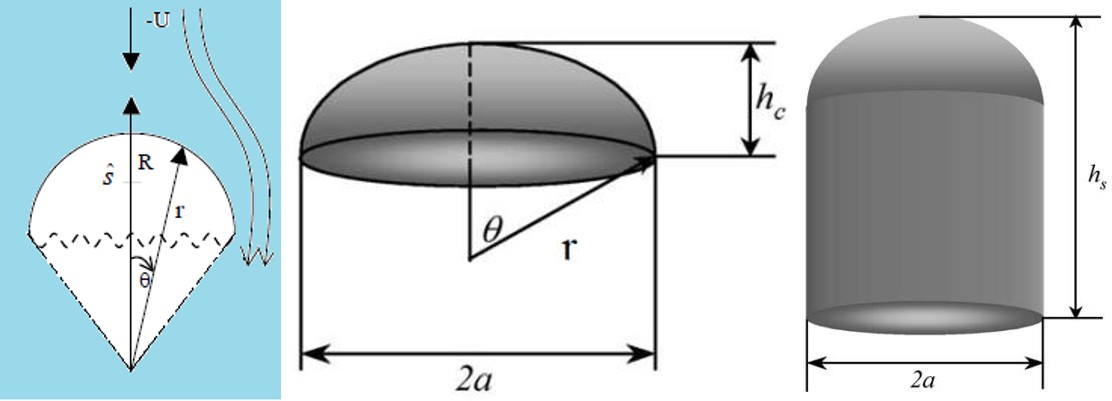
$$ z = - h (r, \theta) = - \left(R - r (\theta) \cos \theta\right). $$
The velocity field in the gas bubble and the liquid is
derived from a potential
$$ u = \nabla \phi , \nabla^ {2} = 0 $$ The velocity at
$$ z = \infty $$
is -u (against z) and
$$ 1 g = - e _ {z} g. $$
For steady flow $$ \rho u \cdot \nabla u = - \Delta p = - \rho e _ {z} g = - \Delta \Gamma \tag {1} $$ $$ \Gamma = p + \rho g z $$
| | u | 2 |
|---|
2 2 Similarly for the gas, Bernoulli function is
| G | u | 2 |
|---|
(3) Where is an unknown constant. Considering normal stress balance $$ C _ {c} $$ $$ - \llbracket p \rrbracket + 2 \| \mu n \cdot D [ n ] \| \cdot n + \frac {2 \sigma}{r (\theta)} = 0 \tag {4} $$ Where [] [] ( ) ( )L G ⋅ − ⋅ = ⋅
Is evaluated on the free surface ( )
$$ r (\theta) = R \left(1 + s \theta^ {2}\right), \sigma $$ is surface tension, is viscosity and the normal component of rate of strain is given by $$ n \cdot D [ u ] \cdot n = \frac {\partial u _ {n}}{\partial n} $$ [] (5) Using (1), (4) and (5) we obtain $$ - \left[ \left[ \Gamma \right] \right] - \left[ \left[ \rho \right] \right] g h + 2 \left[ \left[ \mu \frac {\partial u _ {n}}{\partial n} \right] \right] + \frac {2 \sigma}{r} = 0 \tag {6} $$ $$ - \llbracket \Gamma \rrbracket - \llbracket \rho \rrbracket g h + 2 \left[ \left[ \mu \frac {\partial u _ {n}}{\partial n} \right] \right] + \frac {2 \sigma}{r} = 0 $$ Where –h is the value of z on the free surface.
Assuming that u may be approximated near the stagnation point on the bubble, which is nearly spherical, $$ b = - U r \cos \theta \left(1 + \frac {R ^ {3}}{2 r ^ {3}}\right) $$
3
2 1 cos r R Ur θ φ (7)
φ denotes the potential for a spherical nose. For the liquid, the form ofφin the gas can be neglected. From (7) we compute − − = ∂ ∂ = r R U r ur (8) θ φ cos 1 3
3
+ = ∂ ∂ = 3
r R U r u θ φ θ θ (9)
3
2 1 sin 1
$$\frac{\partial u_n}{\partial n} = \frac{\partial u_r}{\partial r} = -\frac{3UR^3}{r^4} \cos \theta$$
The function (8), (9) and (10) enter into the normal stress balance at $r(\theta) = R(1 + s\theta^2)$. The balance is to be satisfied near the stagnation point, for small $\theta$, neglecting terms that go to zero faster than $\theta^2$. At the free surface,
$$u_r = -U \left\{ 1 - \frac{1}{(1 - s\theta^2)^3} \right\} = -3Us\theta^2, \quad u_\theta = \frac{3}{2}U\theta$$
$$\frac{\partial u_n}{\partial n} = -\frac{3U \left( 1 - \frac{1}{2}\theta^2 \right)}{R(1 + s\theta^2)^4} = -\frac{3U}{R} \left\{ 1 - \left( 4s + \frac{1}{2} \right)\theta^2 \right\}$$
$$u_r^2 = 0$$
$$u_\theta^2 = \frac{9}{8}U^2\theta^2$$
$$h = R - r\cos \theta = R - R(1 + s\theta^2)\left( 1 - \frac{1}{2}\theta^2 \right) = R\left( \frac{1}{2} - s \right)\theta^2$$
The motion of the gas in bubble is not known but it enters into (6) as the coefficient of $\rho_G$ and $\mu_G$, which are small relative to the corresponding liquid terms. Evaluating (2) and (3) on the free surface, with gas motion zero, we obtain,
$$\Gamma = -\frac{9}{8}\rho U^2\theta^2 + \rho \frac{U^2}{2}$$
$$\Gamma_G = C_G$$
Using (11) to (16), we may rewrite
$$0 = -C_G + \Gamma + (\rho - \rho_G)gh - 2\mu \frac{\partial u_r}{\partial r} + \frac{2\sigma}{r}$$
$$C_G = \frac{\rho U^2}{2} - \frac{9}{8}\rho U^2\theta^2 + (\rho - \rho_G)g\left( \frac{1}{2} - s \right)R\theta^2 + \frac{6\mu}{R} \left\{ 1 - \left( 4s + \frac{1}{2} \right)\theta^2 \right\} + \frac{2\sigma}{R}\left( 1 - s \theta^2 \right)$$
The constant terms vanish
The coefficient of $\theta^2$ also vanishes:
$$\frac{9}{8}\rho U^2 + \frac{3U\mu}{R} + \frac{24sU\mu}{R} = (\rho - \rho_G)g\frac{R}{2} - s \left\{ (\rho - \rho_G)gR + \frac{2\sigma}{R} \right\}$$
$$\frac{9}{8}\rho U^2 - (\rho - \rho_G)\left( \frac{1}{2} - s \right)gR + \frac{6U\mu}{R}\left( 4s + \frac{1}{2} \right) + \frac{2\sigma}{R} = 0$$
The general solution of (19) with $D = 2R$ is
$$U = \frac{8v(1 + 8s)}{D} + \frac{\sqrt{2}}{3}\left[ (1 - 2s)gD \frac{\rho - \rho_G}{\rho} - \frac{16s\sigma}{\rho D} + \frac{32v^2}{D^2}(1 + 8s)^2 \right]^{\frac{1}{2}}$$
It is convenient to write (20) in a dimensionless form:
$$Fr = -\frac{8(1 + 8s)}{3\Re_G} + \frac{\sqrt{2}}{3}\left[ \frac{(1 - 2s)(\rho - \rho_G)}{\rho} - \frac{16s}{Eo} + \frac{32}{\Re_G^2}(1 + 8s)^2 \right]^{\frac{1}{2}}$$
$$Fr = \frac{U}{\sqrt{gD}}$$, Froude number
$$\Re_G = \frac{\sqrt{gD^2}}{v}, \text{Gravity Reynolds number}$$
$$Eo = \frac{(\rho - \rho_G)gD^2}{\sigma}, \text{Eotvosb number}$$
Calculation of Deviation from Sphericity
From the geometrical definition of 2nd derivative we can write
$$s = \frac{\left( r_1 - r_2 \right) - 2R}{\Delta\theta^2}$$
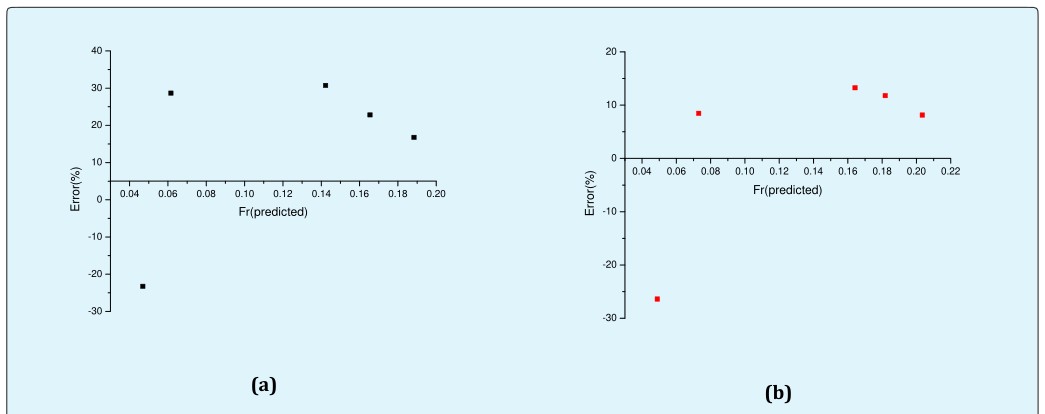
Where $r_1, r_2$ and $R$ are the radius $\Delta\theta$ and is the angle shown in Figure 3 Analyzing the actual profile of the nose of a Taylor bubble, one can easily find out the parameters $r_1, r_2, R$ and $\Delta\theta$. For this purpose we have captured the photograph of a Taylor bubble and analyzed by Image-Pro Plus software (version 5.1) to get the actual shape of the bubble [10, 11, 12, 13]. The above parameters have measured geometrically and using these values "s" has been calculated. Putting the value of "s" obtained from above analysis the Equation (21) gives satisfactory results, which are shown in Table 4.5. The % deviation is shown in table, which is calculated based on the experimental value of rise velocity.
$$s = \frac{\left( r_1 - r_2 \right) - 2R}{\Delta\theta^2}$$
- Empirical Correlations to Predict Rise
- Velocity of Taylor bubble
- A thorough survey of the past literature has revealed that several correlations have been proposed by the past
- D(mm)
- Re
- Eo
- Expt Fr
- Predicted Fr from
- % error
- Eq 1
- Eq 2
- Eq 1
- Eq 2
- 6
- 1454.75
- 4.899114
- 0.036
- 0.04691
- 0.04891
- -23.2573
- -26.3954
- 6.5
- 1640.336
- 5.749654
- 0.07923
- 0.061586
- 0.073059
- 28.64895
- 8.446598
- 8.5
- 2452.965
- 9.83224
- 0.186
- 0.142288
- 0.164213
- 30.72079
- 13.26766
- 9
- 2452.965
- 11.02301
- 0.203235
- 0.165509
- 0.181832
- 22.79393
- 11.77076
- 9.5
- 2898.33
- 12.28181
- 0.22
- 0.188418
- 0.203491
- 16.76161
- 8.112943
Table 3: The prediction of rise velocity from equations 1-2.
| Surface of the cap | D(mm) | S | Fr | Re | Eo |
|---|---|---|---|---|---|
| Image 1 | 6 | 0.1879 | 0.036 | 1454.75 | 4.899114 |
| Image 2 | 6.5 | 0.20431 | 0.07923 | 1640.336 | 5.749654 |
| Image 3 | 8.5 | 0.235004 | 0.186 | 2452.965 | 9.83224 |
| Image | 9 | 0.2443 | 0.203235 | 2672.55 | 11.02301 |
| Image | 9.5 | 0.2536 | 0.22 | 2898.33 | 12.28181 |
Table 5: Calculation of sphericity “s”.
| D(mm) | Re | Eo | S | Fr (Eq1) | Expt Fr | % error |
| 6 | 1454.75 | 4.899114 | 0.1879 | 0.041 | 0.036 | -12.1951 |
| 6.5 | 1640.336 | 5.749654 | 0.20431 | 0.06571 | 0.07923 | 20.57525 |
| 8.5 | 2452.965 | 9.83224 | 0.235004 | 0.17757 | 0.186 | 4.747424 |
| 9 | 2672.55 | 11.02301 | 0.2443 | 0.1817 | 0.203235 | 11.85195 |
| 9.5 | 2898.33 | 12.28181 | 0.2536 | 0.186 | 0.22 | 18.27957 |
Table 6: Comparison of predicted results with experimental results.
5. Hills JH, Chety P (1998) The rising velocity of Taylor
bubbles in an annulus. Chem Engng Res Des 76(6): 723-727.
6. Van Hout R, Gulitski A, Barnea D, Shemer L (2002)
Experimental investigation of the velocity field induced by a Taylor bubble rising in stagnant water. Intl J Multiphase Flow 28(4): 579-596.
There is no movement of Taylor in 5 mm diameter tube because surface tensional force is dominated in small channel. Predicted shape of the Taylor bubble obtained from potential flow theory agrees with actual shape obtained from image analysis within sufficient accuracy. Propagation rate has been predicted from viscous potential theory. Deviation from sphericity is also incorporated into the analysis.
References
-
Fabre J, Line A (1992) Modeling of two-phase slug flow. Annu Rev Fluid Mech 24: 21-46.
-
Garabedian PR (1957) On steady state bubbles generated by Taylor instability. Proc R Soc Lond A 241: 423.
-
Haberman WL, Morton RK (1956) An experimental study of bubbles moving in liquids. Trans Am Soc Civil Engng 121: 227-252.
-
Dumitrescu DT (1943) Stromung and Einer Luftbluse in Senkrechten rohr. Z Angew Math Mech 23: 139- 149. Investigation of slug flow Characteristics in the valley of a hilly-terrain pipeline. Int J Multiphase Flow 31(3): 337-357.
-
Bugg JD, Saad GA (2002) The velocity field around a Taylor bubble rising in a stagnant viscous fluid: Numerical and experimental results. Int J Multiphase Flow 28(5): 791-803.
-
Brown RAS (1965) The mechanics of large gas bubbles in tubes. I. Bubble velocities in stagnant liquids. The Can J Chem Eng 43(5): 217-223.
-
Damianides CA, Westwater JW (1988) Two-phase flow patterns in a compact heat exchanger and in small tubes. In Proc 2nd UK Natn Conf on Heat Transfer, pp: 1257-1268.
-
Barajas AM, Panton RL (1993) The effects of contact angle on two phase flow in capillary tubes. Int J Multphase Flow 19(2): 337-346.
-
Takamasa T, Hazuku T, Hibiki T (2008) Experimental Study of gas–liquid two-phase flow affected by wall surface wettability. International Journal of Heat and Fluid Flow 29(6): 1593-1602.
-
Polonsky S, Shemer L, Barnea D (1999b) The relation between the Taylor bubble motion and velocity field ahead of it. Int J Multiphase Flow 25(6-7): 957-975.
-
Bretherton FP (1961) The motion of long bubbles in tubes. J Fluid Mech 10(2): 166-188.
- Nigeria’s Vulnerability in the Face of Global Energy Policy
- A Simulation Study of Investigation of Optimum Oil Production Performance by Applying Various Gas Injection Methods in Oil Reservoir
- Characterization of Permo-Triassic Reservoirs through Thermal Maturity Assessment of Westphalian Source Rocks in the Cheshire Basin
- Influence of Microwax on the Rheological and Thermal Behaviour of a Wax Crude Oil
- Real-Time Monitoring and Performance Optimization of Steam Injection in Heavy Oil Reservoirs Using Fiber Optic Sensing and Integrated Predictive Simulation Models
- Rapid On-Site Determination of the Total Petroleum Hydrocarbon Content of Soils by Handheld Fourier Transform Near-Infrared Spectroscopy: Development of a Global, Site- and Scanner- Independent Calibration Model