Development of a Simplified Foam Hydraulic Model for Vertical Well Drilling
The objective of this work is to propose a simplified foam hydraulic model to be used to predict and simulate foam static and dynamic properties in spite of its simplicity, as well as adequate hole cleaning in vertical wells. Despite its simplicity, the model takes into account the real and actual conditions of the annular constituents. Thus, the analysis of the effects of the annular cuttings (drilled solids) and fluid influx are taken into account in the development of the model. If the foam flow inside the string is considered two-phase (injected liquid and gas), the annular stream is considered a three-phase fluid containing liquids (injected water, liberated water and oil from the drilled cuttings and water and oil influx from the formations), gases (injected gas, liberated gas from the drilled cuttings and gas influx from the formations) and drilled solids. Cuttings slip velocity and hindered cuttings terminal velocities are also taken into account for the adequate and accurate hole cleaning and for the analysis of the cuttings distribution profile along the vertical well. Results obtained from the proposed model revealed that foam hydraulics and rheological properties were affected by the injection pressure. The model was evaluated by running it on two foam-underbalanced wells in the Middle East with absolute average errors (on the downhole pressure at a given depth) less than 2.6 and 10.9% for the first and second wells, respectively. The model accuracy was also compared with those of other models: Valco and Economides’ model and Sporker’s model. The model accuracy nearly equaled that of Valco and Economides’ one whereas it was less than that of Sporker.
Introduction
Foam is commonly used for underbalanced drilling (UBD) because of its low variable density; which makes its adjustment possible to maintain the control of the circulating bottomhole pressures. Foam is also a good UBD drilling medium because of its high effective viscosity; which gives it a superior cuttings lifting and transport ability. It is also used, as a drilling fluid, to transport formation fluids that enter the borehole during UBD operations. This paper is intended to propose an improved computer program using VISUAL BASIC programming language that can be used to better simulate and predict the foam hydraulics for vertical wells.
The objectives of the paper are to develop a simplified hydraulic model that can be used to better understand the hydrodynamics of drilling foam in vertical wells. The model is capable of simultaneously studying and analyzing the effects of the injection parameters (injection pressure and fluid rates) on the circulating pressure and other foam properties such as foam mean velocity, quality, density, viscosity, power and consistency indices, Reynolds number, friction factor as well as the annular cuttings concentration. The values of these parameters can be simultaneously calculated at any required point along the entire sections of the string and the annulus so that the entire well is monitored and controlled during the foam drilling operation. The model simplicity resides in fact that only the differential equation for the principle of the linear momentum conservation coupled with some other published closure expressions is used to build the model. The model starts calculating the hydrodynamics parameters downward inside the drill string, around the bit, and upward in the annulus, thus, the optimum values of the required injection pressure and fluid flow rates can be estimated once the conditions of adequate cuttings removal are satisfied.
Several proposed models of the foam rheology have been published in the literature with different contradictory conclusions Baris O, Ramadan, Osunde O [1, 2, 3]. In fact, the disagreement between the researchers over the adoption of a unique exact flow type of the foam results in the necessity to extensively conduct more detailed studies on foam to determine the ranges of occurrence of each flow type (conditions at which it is considered Bingham-plastic fluid, power-law fluid, yield- power-law fluid, etc.). In correspondence with these challenges, this paper is intended to propose an improved hydraulic model to address the hydraulics, rheological characterizations, and cuttings transport with foam fluids for vertical wells.
Conclusions of Sanghani and Ikoku’s works [1, 4] revealed that at a given foam quality (foam quality is defined as the ratio between the gaseous phase volume at a given temperature and pressure and the total mixture volume at the same condition of temperature and pressure), the foam effective viscosity decreased with increasing shear rates up to the shear rate value of 1000 1/s.
Several Authors reported the works of Okpobiri and Ikoku [1, 2, 5, 6] that predicted the minimum volumetric requirements for foam drilling operations. They assumed that all foam drilling operations were performed in the laminar region, and that foam qualities varied with varying pressures between 0.55 and 0.96.
Ozbayoglu, et al. [7] compared six different rheological models with the data obtained from their experiments. They observed that foam behaved as a power-law fluid at lower qualities and as a Bingham plastic fluid for qualities above 90%.
Ibizugbe [8] concluded that, in spite of previously reported limitations of oil-based drilling foam stability, his study showed that, with the selection of appropriate surfactants and oil, stable oil-based foam could be produced for drilling applications.
Development of the Hydraulic Model
To build a realistic hydraulic model that could be practically applicable in foam drilling operations, the following assumptions are adopted in this paper:
- Foam is considered a homogeneous Non-Newtonian fluid with a rheology that can be dominantly represented as a power-law fluid [4]. It has also been concluded in the literature that the Bingham plastic approach should be adopted at higher qualities [7].
- Foam flow in the drill string is considered a steady state flow of two-phase, in which the gaseous phase is compressible and the liquid phase is considered incompressible, whereas in the annulus, it is considered a steady state flow of three-phase in which the gaseous phase is compressible, and liquids and solids are considered incompressible.
- Well inclination, θ is always less than or equals to the first critical inclination θc1 which is considered to be around 10 degrees [9].
- The temperature in the annulus can be assumed based on the geothermal gradient of the region and, consequently, the temperature inside the drillstring is also calculated neglecting the thermal effects of the steel pipe separating the inside of the drillstring from the annulus.
- In the annular upward flow, foam, formation influx and cuttings are assumed to mix into a uniform homogeneous suspension.
6. For the developed model, the downward and upward flow path of each section is divided into equal grid cells, ΔZ, and starting from the first grid cell inside the string, all required calculations are performed down to the drill bit and up the annulus till the surface, and the total pressure drop is the summation of all grid cells.
The linear momentum (T) of a particle with a mass (m) moving with a velocity (U) is defined to be the product of the mass and the velocity [10]:
M = m .U. (1)
Using Newton’s second law of motion, it will be easier to relate the linear momentum of a particle (M) to the resultant force (F) that is acting on the particle with acceleration (a) as follows:
$$ \mathrm {F} = \mathrm {m . a} = \frac {\mathrm {d U}}{\mathrm {d t}} = \frac {\mathrm {d} (\mathrm {m U})}{\mathrm {d t}} \tag {2} $$ The external forces acting on a foam system are: 1- fluid weight; 2- shear forces; and: 3- pressure forces. Applying the Newton’s second law on a unit fluid volume results in: (Fluid weight force + Shear force + Pressure force) = dM +Totalacceleration dt (3) d(m U2) g
4τw dP d(m U)
dt Where: gc is the Newton’s law conversion factor (ft-
$$ \mathrm {l b} _ {\mathrm {m}} / \mathrm {l b} _ {\mathrm {f}} - c u t i t i n g s = s o l i d s +. $$
+ sec2); θ is the hole inclination in degrees. The ratios of the wetted perimeter (S) to the cross sectional areas of the string and annulus are, respectively:
4 𝜋 𝐷𝑝𝑖𝑝𝑒
𝑆
4 𝐴𝑝𝑖𝑝𝑒 =
𝜋 𝐷𝑝𝑖𝑝𝑒2 =
𝐷𝑝𝑖𝑝𝑒 (5)
𝑆
4 (𝜋 𝐷ℎ𝑜𝑙𝑒+ 𝜋 𝑂𝐷𝑝𝑖𝑝𝑒)
4 𝜋 (𝐷ℎ𝑜𝑙𝑒+ 𝑂𝐷𝑝𝑖𝑝𝑒)
𝐴𝑎𝑛𝑛 =
2 ) = 𝜋 (𝐷ℎ𝑜𝑙𝑒+ 𝑂𝐷𝑝𝑖𝑝𝑒)(𝐷ℎ𝑜𝑙𝑒− 𝑂𝐷𝑝𝑖𝑝𝑒)
2 − 𝑂𝐷𝑝𝑖𝑝𝑒
𝜋 (𝐷ℎ𝑜𝑙𝑒
4 = (𝐷ℎ𝑜𝑙𝑒− 𝑂𝐷𝑝𝑖𝑝𝑒) (6)
Then, substituting these ratio values and taking into account the negative sign for the annular flow direction:
d(m U2)
dP g S τw Aann −
dZ = −ρf dZ (7) gc cos (θ) −
As in the steady state condition of the foam underbalanced drilling, the difference in foam velocity is so marginal that the force due to the total acceleration are neglected; the final form of the equations for the string and annular flows, respectively, become:
dP g S τw Apipe (8)
dZ = ρf gc cos(θ) +
dP g S τw Aann (9)
dZ = −ρf gc cos (θ) −
7. The iterative procedures are used to calculate the pressure drop of each grid cell in the drill string using the developed equations. The first and second terms of the right hand side of Equations 8 and 9 denote for the gravitational and frictional components of the pressure drops, respectively. In power law model, the shear stress (τ) is related to shear rate (γ) by the following expression [11]:
n τ + kγ (10) where k and n are flow power index and consistency index, respectively. Inside the drill string: Foam quality Γ at a given pressure P and temperature T is calculated as:
Ug(P & 𝑇) Ug(P & 𝑇)+UL =
Qg(P & 𝑇) Qg(P & 𝑇)+QL (11)
Γ =
Foam density _ρ_f at a given pressure and temperature is calculated using Baris O, Osunde O, Cheng R [1, 3, 9]:
ρf = Γρg(P & T) + (1-Γ) ρL (12) Foam power index (n) and consistency index (k) at a given pressure and temperature can be calculated using Li’s correlations [1, 3, 12]. Specific volume expansion ratio (εs), slip velocity (Uslip), slip coefficient (βc) and wall shear stress (τw), respectively, at a given point can be calculated.
ρL εs = ρf (13a) Uslip =
βcτw IDstring (13b)
0.552τw −0.847
0.247τw −0.559 βc = εs0.36 (for stiffer foam) =
εs−0.173 (for non- stiffer foam) (13c)
Petroleum & Petrochemical Engineering Journal
$$\tau_w = \frac{\bar{F} \cdot 1D_{\text{string}}}{4 \Delta Z} = k \gamma^n = k \left( \frac{8 U}{1 D} \right)^n \tag{13d}$$
The corrected foam flow rate ($Q_f = Q_L + Q_s$) is calculated, and the corresponding foam velocity is also calculated using:
$$\left( U_f = \frac{Q_f}{A_{\text{string}}} - U_{\text{slip}} \right) \tag{13e}$$
Foam effective viscosity $\mu_f$ [1, 3, 4] is calculated using the following equation:
$$\mu_f = k \left( \frac{3n+1}{4n} \right) \left( \frac{8 U_f}{1 D} \right)^{n-1} \tag{14}$$
The Reynolds Number $R_f$ [3] is calculated using the following equation:
$$R_f = \frac{8^{1-n} \rho_f U_f^2 - n I D^n}{k_f \left[ \frac{3n+1}{4n} \right]^n} \tag{15}$$
The bit pressure drop $\Delta P_{\text{bit}}$ is calculated using the iterative procedures and equation proposed by Okpobiri and Ikoku [1, 5].
In the annulus: The pressure drop in the annular grid cell is calculated using the developed equation:
$$\frac{dP}{dZ} = -\rho_f \frac{g}{g_c} \cos(\theta) - \frac{S \tau_w}{A_{\text{ann}}} \tag{9}$$
To effectively use Equation9 for pressure calculations in the annulus, the following steps are followed:
Calculate the reservoir fluid volumetric rates, $Q_i$, entering the annular stream due to the disintegration of the reservoir rocks [13]:
$$Q_i = A_{\text{hole}} \cdot ROP \cdot f \cdot Sat_i \quad i = \text{water, oil and gas.} \tag{16}$$
Where, ROP, $A_{\text{hole}}$, $\phi$ and Sat are rate of penetration ($ft/hr$), hole cross sectional area ($ft^2$), formation porosity (fraction) and fluid pore saturation (fraction), respectively.
Calculate, respectively, the solids and annular flow rates due to the rock disintegration using:
$$Q_{\text{solids}} = A_{\text{hole}} \cdot ROP \cdot (1 - f) \tag{17a}$$
$$Q_{\text{ann}} = A_{\text{hole}} \cdot ROP \tag{17b}$$
Calculate the foam flow rate at the annular conditions of temperature and pressure:
$$Q_f(\text{ann}) = Q_{\text{g. ann P, T}} + Q_L(\text{ann}) \tag{18}$$
Calculate the approximated cuttings concentration in the annulus using:
$$CC_{\text{approx}} = \frac{Q_{\text{solids}}}{Q_{\text{ann}} + Q_f(\text{ann})} \tag{19}$$
Calculate the assumed annular mixture density:
$$\rho_{\text{ann(ass)}} = \rho_f \times \left( 1 - CC_{\text{approx}} \right) + \rho_{\text{solids}} \times CC_{\text{approx}} \tag{20}$$
Calculate the following parameters:
$$\Delta T = \text{GG x } \Delta Z \tag{21}$$
$$\Delta P_{\text{guessed}} = \text{Constant } x_{\text{ann(ass)}} \times \Delta Z \tag{22}$$
Calculate the average temperature, $\bar{T}$, and average pressure $\bar{P}$ in the annular grid cell j:
$$T_2 = T_{j-1} - \Delta T \tag{23a}$$
$$\bar{T} = T_{j-1} - 0.5 \Delta T \tag{23b}$$
$$P_2 = P_{j-1} - \Delta P_{\text{guessed}} \tag{23c}$$
$$\bar{P} = P_{j-1} - 0.5 \Delta P_{\text{guessed}} \tag{23d}$$
Calculate influx rates of reservoir fluids, $Q_{\text{influx(i)}}$, using the modified Vogel’s method [14] in case of depleted-drive reservoirs in which the average reservoir pressure, $P_{\text{res}}$, is less than the bubble-point pressure.
Calculate the mass flow rates of the reservoir water, oil and solids:
$$\dot{m}_1 = \left[ Q_{\text{i}} + Q_{\text{influx(i)}} \right] \times \rho_{\text{i}} \tag{24}$$
$$\dot{m}_{\text{solids}} = Q_{\text{solids}} \times \rho_{\text{solids}} \tag{25}$$
Calculate the corrected gas flow rates, i.e.: the injected gas $Q_{g(inj)}$, $Q_{g}(g)$ entering the annular stream due to the disintegration of the reservoir rocks and $Q_{influx}(g)$. These corrections are due to the changes of the gas volume due to the pressure and temperature changes [3].
Calculate the molecular weight of the annular foam gases:
$$Mwt_{(ann)} = Mwt_{(inj)} \times \frac{Q_{g(inj,corr)}}{Q_{g(inj,corr)} + Q_{g(corr)} + Q_{influx(g,corr)}} + Mwt_{(influx)} \times \frac{Q_{g(inj,corr)} + Q_{influx(g,corr)}}{Q_{g(inj)} + Q_{g(corr)} + Q_{influx(g,corr)}} \dots$$ (26)
Where: $Mwt_{(inj)}$, $Mwt_{(influx)}$ and $Mwt_{(ann)}$ are the injected gas molecular weight, reservoir gases molecular weight and average annular gases molecular weight, respectively.
Calculate the critical temperature ($T_c$), critical pressure ($P_c$), pseudo-reduced pressure ($P_r$) and pseudo-reduced temperature ($T_r$) of the annular mixture gases.
Calculate the compressibility factor ($Z_2$) of the gaseous phase in foam using the methods described by Kingdom KD [15].
Calculate the annular corrected foam density, $\rho_f(ann)$, using Osunde O [3]:
$$\rho_f(ann) = \frac{Q_{tot}(ann)}{Q_{tot(ann)}}$$ (27)
Calculate the corrected annular cuttings concentration, CC:
$$CC = \frac{Q_{solids}}{Q_{tot(ann)}}$$ (28)
Calculate the annular foam quality ($\Gamma_{ann}$):
$$\Gamma_{ann} = \frac{Q_{g(inj,corr)} + Q_{g(corr)} + Q_{influx(g,corr)}}{Q_{tot(ann)} - Q_{solids}}$$ (29)
Calculate the density of the mixture of the reservoir gas within the foam by the use of the real gas equation of state as follows:
$$\rho_g(ann) = \frac{FMwt(influx)}{RZT}$$ (30)
Calculate the total mass flow rate of the reservoir gases $m_g$:
$$m_g = \left( Q_{g(corr)} + Q_{influx(g,corr)} \right) x \rho_g(ann)$$ (31)
Calculate the cuttings mass flow rate $m_{cuttings}$:
$$m_{cuttings} = m_{solids} + \sum \dot{m}_i$$ (32)
Calculate the average cuttings density $\rho_{cuttings}$:
$$\rho_{cuttings} = \frac{m_{cuttings}}{Q_{ann}}$$ (33)
Calculate the annular mixture density $\rho_{mixture}$ [1]:
$$\rho_{mixture} = \frac{\rho_{cuttings} + m_{cuttings} + \rho_f(m_f)}{m_{cuttings} + m_f}$$ (34)
Calculate flow consistency (K) and the flow behavior (n) indices using Li’s correlations [12].
Calculate the annular gross velocity:
$$U_{ann(gross)} = \frac{Q_{tot(ann)}}{A_{ann}}$$ (35)
Calculate the annular foam effective viscosity, $\mu_f(ann)$ using Baris O, Sanghani V [1, 4]:
$$\mu_f(ann) = K \left( \frac{2n+1}{3n} \right) \frac{12U_{ann(gross)}}{D_{hole} - OD_{string}}^{n-1}$$ (36)
Where: $D_{hole}$ denotes for the diameter of the wellbore (ft) and OD denotes for the string outside diameter inside the wellbore (ft).
Calculate the uncorrected particle setting velocity, $U_{sett}$, using the equation developed by Moore [16].
Calculate the particle Reynolds Number ($Re_p(sett)$) using the uncorrected particle settling velocity and the corresponding drag coefficient $C_D$ [17, 18, 19].
Calculate the corrected settling (terminal) velocity $U_{term}$ [3, 20, 21]:
$$U_{term} = \sqrt{\frac{4 g_c D_{solids}}{3 C_D} \left( \frac{\rho_{solids} - \rho_f(ann)}{\rho_f(ann)} \right)}$$ (37)
Calculate the hindered terminal velocity, $U_h$, using the iterative procedures. If the settling is carried out with high concentrations of solids in the fluid so that the particles are so close together that collision between the particles is practically continuous and the relative fall of particles involves repeated pushing apart of the lighter by the heavier particles it is called “Hindered Settling or Hindered Velocity” [3, 21]. Calculate the annular mixture velocity Uann [9]:
Uh ρsolids CC
Uann = Uann(gross) -
ρmixture (38) Calculate the annular mixture Reynolds Number, Reann [1]: Calculate Darcy friction factor ff [22]: ff =
64 𝑅𝑒𝑓 For Ref ≤ 2100 (Laminar flow for both string and annulus) (39a) For Ref ˃ 2100 (Turbulent flow), a modified Colebrook’s correlation proposed by Chen [1, 23] is used to calculate the friction factor as:
1.1098 (roughness )
1 roughness
5.0452 dh $$ \sqrt {\frac {1}{f _ {\mathrm {f}}}} = - 4 \log \frac {r _ {\mathrm {f}}}{3} $$ Ref log (
3.7065dh −
2.8257 + √
5.8506 Ref0.8981)] (39b)
Calculate the shear stress τ [9].
Equations (8 and 9) represent first-order ordinary differential equations that describe the hydrodynamics of foam flow. Pressure is the principal unknown of the equation. This paper implements the method proposed by Cash-Karp Embedded Runge-Kutta procedure [1, 24]. To solve Equations (8 and 9) for the pressure (P), vector version of Cash-Karp (K1 through K6) are calculated and used for the solution of the pressure.
Finally, check for the hole cleaning condition [9]:
FB + FD cos (θ) + FLif sin (θ) > FG (40) Where: FB, FD, FLif and FG are the buoyant, drag, lift and gravitation forces, respectively.
Results and Discussions
Simulated Effects of the Injection Pressure on the Pressure Drops
Figure 1 shows that the pressure drop inside the drillstring increases with the increase of the injection pressures. At 1,000 lbf/in2 (psia) of the injection pressure, the pressure increases slightly to 1,500 lbf/in2 at the bottom of the well before the bit, whereas, it increases to 4,287 lbf/in2 at an injection pressure of 3,000 lbf/in2 (Figure1). The annular pressure decreases from 1,280 lbf/in2 at the annular bottom to 630 lbf/in2 at the surface for an injection pressure of 1,000 lbf/in2, whereas it decreases from 2,784 lbf/in2 at its bottom to 1,610 lbf/in2 at the surface for the injection pressure of 2,000 lbf/in2, and decreases from 4,173 lbf/in2 at the annular bottom to 2,602 lbf/in2 at the surface for the injection pressure of 3,000 lbf/in2 (Figure1). It is worthy to observe that the pressure profiles for the given conditions in Table 1 are not significantly affected by the drillstring and annular geometries as each pressure curve/line has a nearly constant slope from the surface to the bottom. This means that the dominant component of the pressure drop is the hydrostatic component, and that the frictional component has minor effects on the pressure profile. Figure1 shows the effect on the injection pressure on both string and annulus on the same plot. The differences between the values of the string bottom pressures and those of the annulus bottom represent the bit pressure drops for the respective three injection pressure.
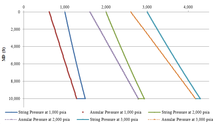
Figure1: Simulated effects of injection pressure on foam pressure drops in the string and annulus.
| Surface Conditions | Surface pressure (psia) | 14.7 |
|---|---|---|
| Surface temperature (°F) | 60 | |
| Injection Conditions | Injection pressure (psia) | variable |
| Injection temperature (°F) | 65 | |
| Injection liquid rate (gal/min) | 5 | |
| Injection gas rate (scf/min) | 2,000 | |
| Well Data | Total depth (measured) (ft) | 10,000 |
| Last casing size (in.) | 9.25 x 8.68 | |
| Last casing depth (measured) (ft) | 7,000 | |
| Temperature gradient (°F/ft) | 0.015 | |
| ROP (ft/hr) | 30 | |
| Formation Data | Porosity, % | 25 |
| Rock density (lbm/gal) | 20 | |
| Formation water density (lbm/gal) | 8.5 | |
| Formation oil density (lbm/gal) | 6 | |
| Formation gas molecular weight (lbm/lb ) mole | 22 | |
| Formation water saturation (%) | 40 | |
| Formation oil saturation (%) | 30 | |
| Formation gas saturation (%) | 30 | |
| Drillstring Geometry | Drillpipe ID (in.) | 4.27 |
| Drillpipe OD (in.) | 5 | |
| Drillpipe length (ft) | 9,000 | |
| HWDP ID (in.) | 3 | |
| HWDP OD (in.) | 5 | |
| HWDP length (ft) | 500 | |
| Drill collar ID (in.) | 2.25 | |
| Drill collar OD (in.) | 6 | |
| Drill bit | Nozzle diameters (in.) | 3 x 13/32 |
| Foam | Water + Nitrogen |
Table 1: Input data for the foam drilling program.
Simulated Effects of the Injection Pressure on the Foam Velocity
The increase of the injection pressure decreases the foam velocity in the string (Figure 2) as well as in the annulus. In the drillstring for example, the effects of the injection pressures higher than 3,000 lbf/in2 are not significant on the velocity profile as foam velocity decreases very slightly.
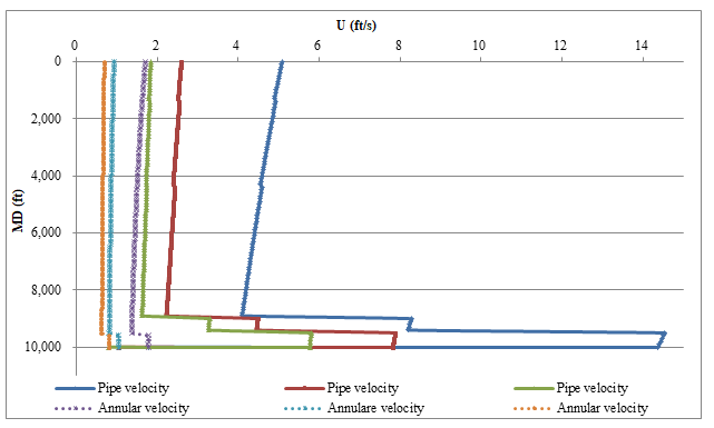
The velocity decreases from 4.99 ft/s to 1.83 ft/s when the injection pressure is increased from 1,000 to 3,000 lbf/in2. For the annular mixture velocity (Figure 2), the same conclusion is also noticed. The reason for the minor change of the velocity at higher injection pressures is that, the pressures cause compressibility of the gaseous phase within the foam. Therefore, further increase of the injection pressures above a limit (3000 lbf/in2 in this particular case) cannot significantly compress the gaseous phase due to the deviation from the ideality, thus, little change is observed in the mixture velocity.
Simulated Effects of the Injection Pressure on the Foam Quality
Foam quality decreases with the increase of the injection pressure in the string and in the annulus (Figure 3).
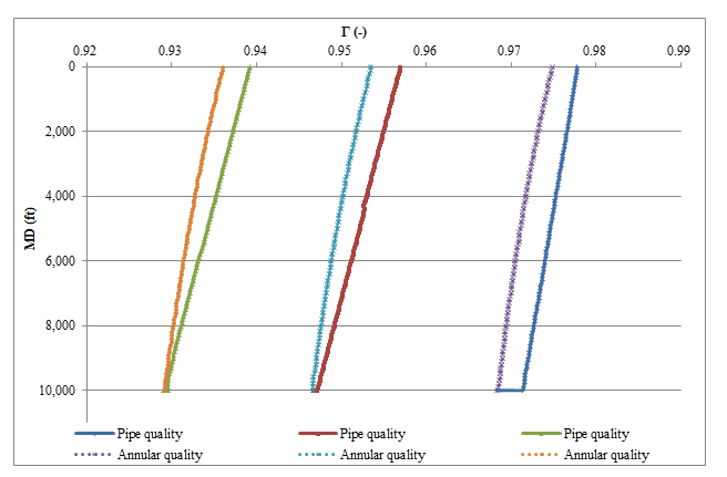
The increase of the injection pressure causes the compressibility and the shrinkage of the gaseous phase within the foam fluid, resulting in the decrease of the foam quality. The effects of the injection pressures are more significant at pressures up to 3,000 lbf/in2. At higher values of the injection pressure, the effects of the injection pressures become less pronounced. This might be interpreted also by the act that at higher pressure values, gas deviation from ideal to real gases becomes more pronounced.
lbm/gal at the injection pressure of 2,000 lbf/in2 to a value of 2.7 lbm/gal at the injection pressure of 3,000 lbf/in2, Figure 4. For the annular flow, the annular mixture density is approximately doubled from 1.1 lbm/gal at an injection pressure of 1,000 lbf/in2 to 2 lbm/gal at the injection pressure of 2,000 lbf/in2. The annular mixture density is also increased from 2 lbm/gal at an injection pressure of 2,000 lbf/in2 to only 2.67 lbm/gal at the injection pressure of 3,000 lbf/in2. It is also worthy to note that, in Figure4, each value of the annular mixture density remains more or less constant along the entire annular section. This is due to the effects of the presence of the formation solids that play the dominant role among both of liquid and gas. As the specific gravity, and hence, density of the drilled solids are much higher than those of the gases and liquids, the annular mixture density becomes dominantly a function of the drilled solids with negligible effects of the other mixture constituents.
Simulated Effects of the Injection Pressure on the Foam Density
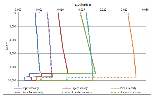
Figure 4 shows the effects of the injection pressures on the foam density in the string as well as in the annulus. Thus, a foam density in the string is doubled from 1 to 2 lbm/gal if the injection pressure is also doubled from 1,000 to 2,000 lbf/in2, whereas it is increased from 2
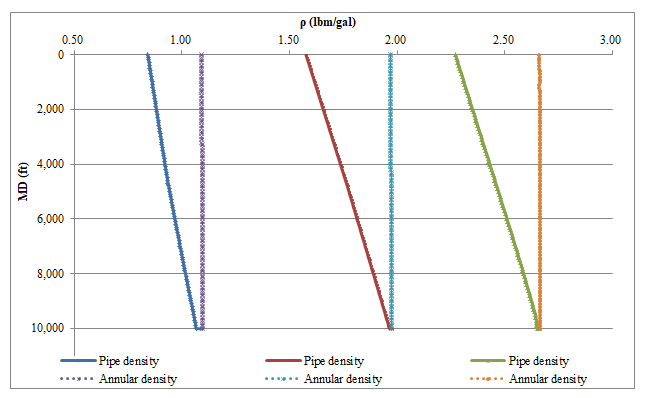
Figure 5 shows that the foam effective viscosity is affected by the injection pressure as its value in the string is increased from 0.005 lbm/ft-s (7 cp) at an injection pressure of 1,000 lbf/in2 to 0.01 lbm/ft-s (15 cp) at the injection pressure of 2,000 lbf/in2. It increases also to 0.017 lbm/ft-s (25 cp) at the injection pressure of 3,000 lbf/in2 (Figure 5). Foam effective viscosity in the annulus increases from 0.008 lbm/ft-s (12 cp) at an injection pressure of 1,000 lbf/in2 to 0.0175 lbm/ft-s (20 cp) at the injection pressure of 2,000 lbf/in2. It increases also 0.0275 lbm/ft-s (41 cp) at the injection pressure of 3,000 lbf/in2. From Figure 5, it is also noted that the effective viscosity is affected by the variation of the drillstring and annular geometries as is the case of the annuli: between 8.5 inches-open hole and 6 inches drill collar; and the annular section between the 8.5 inches-open hole or 8.68 inches- cased hole and 5 inches drillpipe. This is due to the fact that the effective viscosity is a function of the foam velocity and the flow power and consistency indices which have nonlinear relationship with the foam quality.
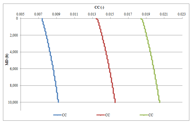
Simulated Effects of the Injection Pressure on the Cuttings Concentration (CC)
Cuttings concentration increases with the increase of the injection pressures (Figure 6). Cuttings concentration can be reduced from 0.0205 (2.05%) at an injection pressure of 3,000 lbf/in2 to 0.008 (0.8%) at the injection pressure of 1,000 lbf/in2 as shown in Figure 6. But the choice of varying and diversifying the values of the injection pressure depends on the required pressure window to be established on the open annulus for the hole control and stability. Lower injection pressures are profitable in point of view of cuttings removal and hole cleaning, but this decision of lowering the injection pressure must be taken after having taken into consideration all factors affecting on the hole stability in order to successfully and optimally carry out the operations of foam underbalanced drilling.
Model Evaluation, Validation and History Matching
- Model Evaluation and Validation with the First
- Field Case Study
- The program has been run using the input data from
- Depth (ft)Pinj (psia)Pactual (psia)Pmodel (psia)PValco-Eco (psia) PSporker (psia) Errormodel (%)ErrorValco-Econ (%) ErrorSporker (%)
- 2,494
- 750
- 989.5
- 983.7
- 956.6
- 986.6
- 0.59
- 3.32
- 0.29
- 2,622
- 780
- 998.5
- 1,040.1
- 958.4
- 995.8
- 4.17
- 4.02
- 0.27
- 3,019
- 880
- 1,252.3
- 1,215.6
- 1207.9
- 1,249
- 2.92
- 3.55
- 0.26
Table 2: Comparison of the bottomhole pressures among the field data, the developed model, Valco-Economides’ model
The results of the comparison between the actual bottomhole pressures obtained from the downhole LWD tools at three different depth points, those of the developed model in this work, those of Valco-Economides’ model and those of Sporker et al.’s model are also shown in Table 2 and graphically represented in Figure 7a & 7b.
The available field data in term of bottomhole pressures have been evaluated and it has been found that the proposed model matches very well the actual result points with an average absolute error percent of 2.56 % compared to 3.63% and 0.27% for Valco-Economides and Sporker et al.’ models, respectively.
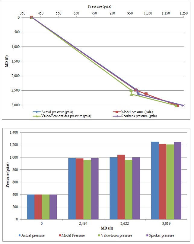
Figure 7a: Comparison of the bottomhole pressure among the actual field data, developed model, Valco-Economides’ model and Sporker’s model for the developed model evaluation and validation with the first well.
Figure 7b: Comparison of the bottomhole pressure among the actual field data, developed model, Valco-Economides’ model and Sporker’s model for the developed model evaluation and validation with the first well.
Model Evaluation and Validation with the Second Field Case Study
The program was also run with the input data of Table 3. The actual field results, those from the developed model, those from Valco-Economides’ model and those from Sporker et al.’s model are also presented in Table 3, and graphically shown in Figure 8a & 8b. From Table 3, it is clear that the convergence between the recorded bottomhole pressures and those of the developed model is less than the convergence between them in case of the first case study. The error percentages of the different depth points are also shown in Table 3; and the overall average absolute error of the developed model is 10.85 % compared to 1.16% and 0.2% for Valco-Economides and Sporker et al.’s models, respectively. So, from these two field cases, it can be concluded that the developed model simulates and predicts well in case of moderate to high gas contents within the foam as was the case for the first well with an average error percentage of 2.56% where the foam quality varied from 81 to 85%. The developed model accuracy might suffer and decrease at low gas contents within the foam as was the case for the second well with an average error percentage of 10.85% where the foam quality varied from 61 to 77%.
| Depth (ft) | Q (gal/min) L | P actual | P model | P Valco-Econl | P Sporker | Error mode | l | Error Valco-Econ | Error Sporker | |||||||||||||
|---|---|---|---|---|---|---|---|---|---|---|---|---|---|---|---|---|---|---|---|---|---|---|
| (psia) | (psia) | (psia) | (psia) | (%) | (%) | (%) | ||||||||||||||||
| 8,202 | 19 | 2,775 | 2,497.1 | 2,732.5 | 2,773 | 10.01 | 1.53 | 0.10 | ||||||||||||||
| 8,243 | 14 | 2,650 | 2,249 | 2,622.5 | 2,646 | 15.13 | 1.04 | 0.15 | ||||||||||||||
| 8,324 | 14 | 2,500 | 2,245 | 2,473.5 | 2,505 | 10.2 | 1.06 | 0.20 | ||||||||||||||
| 8,474 | 14 | 2,500 | 2,267.6 | 2,472.5 | 2,507 | 9.3 | 1.10 | 0.28 | ||||||||||||||
| 8,818 | 14 | 2,600 | 2,349.8 | 2,572.5 | 2,593 | 9.62 | 1.06 | 0.27 |
Table 3: Comparison of the bottomhole pressures among the field data, the developed model, Valco Economides’ model and Sporker’s
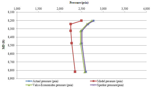
Figure 8a: Comparison of the bottomhole pressure among the actual field data, developed model, Valco Economides’ model and Sporker’s model for the developed model evaluation and validation with the second well.
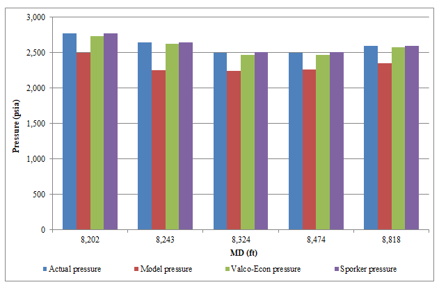
Figure 8b: Comparison of the bottomhole pressure among the actual field data, developed model, Valco Economides’ model and Sporker’s model for the developed model evaluation and validation with the second well.
Conclusions
- Hydraulic model was developed to study and analyze the foam hydrodynamics in vertical wells [27].
- The developed model was used to analyze the effects of the injection pressure on a number of foam rheological properties under the downhole conditions so that the foam drilling operation and its hydraulics are entirely monitored and controlled while drilling with foam [28].
- The developed model simulated well at moderate to high gas contents within the foam fluids, whereas its accuracy might be reduced at low gas contents within the foam fluids.
- Based on two field cases, the developed model accuracy approximately equaled that of the Valco-Economides’ model, but was less than that of Sporker et al. (the best one for both wells).
- The increase of the injection pressure increased the bottomhole pressure, foam density, foam effective viscosity and cuttings concentration; whereas it decreased foam velocity and foam quality.
- The developed model can be used to estimate the optimum injection pressure upon satisfying the hole cleaning conditions [29, 30].
Acknowledgment
The authors would like to express their deepest gratefulness to the Petroleum Engineering Department, Cairo University, for its endless supports during the course of this work.
Nomenclature
a = acceleration, L/t2, ft/s2 [m/s2] A = Cross sectional area, L2, ft2 [m2] b1 1 through b6 6 = constant values proposed by Cash- Karp C = Coefficient, dimensionless CC = Cuttings concentration, fraction [dimensionless] CF = Correction factor, dimensionless D = Diameter, L, in. or ft [m] DA = Annular diameter, L, in. or ft [m] DC = Drill collar, L, in. or ft [m] DP = Drillpipe, L, in. or ft [m] DS = String depth, L, in. or ft [m] DSG = Drillstring, dimensionless F = Force, m-L/t2, lbf [N] ff = Friction factor, dimensionless g = Gravitational acceleration, L/t2, ft/s2 [m/s2] gc = Unit conversion factor, dimensionless (32.174 lbm- ft/lbf-s2) [kg-m/Ns2] GC: Geometry Counter, dimensionless GG = geothermal gradient, °F/ft or °R/ft [°C/m or K/m] H = Thickness, L, ft [m] HWDP = Heavyweight drillpipe, L, in. or ft [m] ID = Inside diameter, L, in. or ft [m] k = flow consistency index, m-tn-2/L, lbf-sn/ft2 [N-sn/m2]
K1 through K6 = vector versions of Cash-Karp m = mass, m, lbm [kg] 𝑚̇ = mass flow rate, m/t, lbm/s [kg/s] M = linear momentum or quantity of motion, m-L2/t2, lbf-ft [N.m] MD = measured depth, L, ft [m] MW = molecular weight of the fluid, (lbm/lbmol n = flow power index, dimensionless OD = Outside diameter, L, in. or ft [m] P = pressure, m/L-t2, lbf/in2 or lbf/ft2 [Pa] 𝑃̅ = average pressure, m/L-t2, lbf/in2 or lbf/ft2 [Pa] Q = volumetric flow rate, L3/t, ft3/s [m3/s] R = universal gas constant, (10.7315 psia-ft3/lbmol-°R) Re = Reynolds number, dimensionless ROP = rate of penetration, L/t, ft/hr [m/s] S = wetted perimeter, L, in. or ft [m] Sat = fluid saturation, fraction T = temperature, ºF, R [ºC, K] TD = Total depth, L, in. or ft [m] U = Velocity, L/t, ft/s [m/s] V = volume, ft3 [m3] Z = Compressibility factor, dimensionless
Greek Letters
εs = Volume expansion ratio, dimensionless βc = slip coefficient Γ = foam quality, fraction ΔP = pressure drop, m/L-t2, lbf/in2 or lbf/ft2 [Pa] ΔZ = Grid cell length, L, ft [m] θ = well inclination from the vertical, degrees [rad] µ = viscosity, m/L-t, lbm/ft-s, cp [kg/m-s] π = pi, 22/7 ρ = density, m/L3, lbm/ft3 [kg/m3] τ = shear stress, m/L-t2, lbf/in2 or lbf/ft2 [Pa] ϕ = average formation porosity, fraction
Subscripts
ann = annular approx = approximated ass = assumed B = buouyant c = constant (gc unit conversion factor), critical D = drag eff = effective (viscosity) f = foam g = gas G = gravitational h = hindered i = fluid (gas, oil, or water) inj = injection L = liquid lift = lifting max = maximum (maximal) n = nozzle o = oil p = particle P = pressure pen = penetrated r = pseudo-reduced res = reservoir sett = settling T = temperature tot = total term = terminal w = at the wall of pipe or annulus wat = water
SI Metric Conversion Factors
bbl x 1.589 873 E-0.1 = m3 bbl/day-psia x 2.307 E-05 = m3/day-Pa cp x 1 E-03 = Pa·s ft x 3.048 E-01 = m ft2 x 9.3 E-02 = m2 ft3 x 2.8317 E-02 = m3 ft3/s x 2.8317 E-02 = m3/s ft/sec2 x 3.048 E-01 = m/sec2 (°F–32)/1.8 = ºC (ºF + 459.67)/1.8 = K gal/min x 6.31 E-05 = m3/sec in. x 2.54 E-02 = m in.2 x 6.452 E-04 = m2 lbf x 4.45 E 00 = N lbf/ft2 x 47.9041 E 00 = Pa lbm x 4.54 E-01 = kg lbm/ft-sec x 1.4914 E 00 = kg/m-sec lbm/ft3 x 16.052 E 00 = kg/m3 lbm/gal x 120.0869 E 00 = kg/m3 lbf/in2 x 6890 E 00 = Pa (lbf/in2)–1 x 1.45 E-04 = Pa–1 scf/min x 4.72 E-04 = m3/sec
References
-
Baris O, Ayala L, Robert WR (2007) Numerical Modeling of Foam Drilling Hydraulics. The Journal of Engineering Research 4(1): 103-119.
-
Ramadan A, Kuru E, Saasen A (2008) Critical Review of Drilling Foam Rheology. Annual Transactions of the Nordic Rheology Society 11.
-
Osunde O, Kuru E (2008) Numerical Modeling of Cuttings Transport with Foam in Inclined Wells. The Open Fuels & Energy Science Journal 1: 19-33.
-
Sanghani V, Ikoku CU (1983) Rheology of Foam and Its Implications in Drilling and Cleanout Operations. J Energy Resour Technol 105(3): 362-371.
-
Okpobiri GA, Ikoku CU (1982) Experimental Determination of Solids Friction Factors and Minimum Volumetric Requirements in Foam and Mist Drilling and Well Completion Operations. Final Report, Fossil Energy, US Department of Energy.
-
Okpobiri GA, Ikoku CU (1986) Volumetric Requirements for Foam and Mist Drilling Operations. SPE Drilling Engineering 1(1).
-
Ozbayoglu ME, Miska SZ, Takach N, Takach N (2000) Cuttings Transport With Foam in Horizontal and Highly Inclined Wellbores. SPE/IADC Drilling Conference. Amsterdam, Netherlands.
-
Ibizugbe NO (2012) Drainage Behavior of oil-Based Drilling Foam Under Ambient Conditions. MS thesis, University of Oklahomam, Norman, Oklahoma.
-
Cheng R, Wang R (2008) A Three-Segment Hydraulic Model for Annular Cuttings transport With Foam in Horizontal Drilling. Journal of Hydrodynamics 20(1): 67-73.
-
Raymond AS, John WJ (2004) Physics for Scientists and Engineers. 6th(Edn.), Thomson Brooks/Cole.
-
Robert FM, Stefan ZM (2011) Fundamentals of Drilling Engineering. Society of Petroleum Engineers, SPE Textbook Series 12.
-
Li Y, Kuru E (2004) Numerical Modelling of Cuttings Transport with Foam in Vertical Wells. J of Canadian Petroleum Technology 44(3).
-
Tarek A (2010) Reservoir Engineering Handbook. 4th (Edn.), Gulf Professional Publishing, Burlington, USA, pp: 1472.
-
Nind TEW (1981) Principles of Oil Well Production. 2nd (Edn.), McGraw-Hill Book Company, Ontario, Canada.
-
Kingdom KD, Oriji B (2012) A new Computerized Approach to Z-Factor Determination. Transnational Journal of Science and Technology 2(7).
-
Moore L (1974) Drilling Practices Manual. 1st (Edn.), Petroleum Publishing Co., Tulsa, Oklahoma, pp: 228- 239.
-
Matijasic G, Glasnovic A (2001) Measurement and evaluation of drag coecient for settling of spherical particles in pseudoplastic fluids. Chem Biochem Eng Quart 15(1): 21-24.
-
Acharya RA (1986) Particle Transport in Viscous and Viscoelastic Fracturing Fluids. SPE Production Engineering. Society of Petroleum Engineers 1(2): 7.
-
Chien SF (1994) Settling Velocity of Irregularly Shaped Particles. SPE Drilling and Completion 9(4): 281-289.
-
Song Z, Wu T, Xu F, Ruijie L (2008) A simple formula for predicting settling velocity of sediment particles. Water Science and Engineering 1(1): 37-43.
-
Doron P, Granica D, Barnea D (1987) Slurry Flow in Horizontal Pipes - Experimental and Modelling. Int J Multiphase Flow 13(4): 535-547.
-
Çengel AY, Cimbala JM (2006) Fluid Mechanics: Fundamentals and Applications. The McGraw-Hill Companies, New York, NY.
-
Chen NH (1979) An Explicit Equation for Friction Factor in Pipe. Ind Eng Chem Fundamen18(3): 296- 297.
-
Cash JR, Karp AH (1990) Cash-Karp 6 stage, combined order 4 and 5 Runge-Kutta scheme. 60(3): 201-222.
-
Valko P, Economides MJ (1992) Volume Equalized Constitutive Equations for Foamed Polymer Solutions. Journal of Rheology 36: 1033-1055.
-
Sporker HF, Trepess P, Valko P, Economides MJ (1991) System Design for the Measurement of Downhole Dynamic Rheology for Foam Fracturing Fluids. SPE Annual Technical Conference and Exhibition, Dallas, Texas.
-
Al-Kayiem AH, Ibrahim MA (2015) The influence of the equivalent hydraulic diameter on the pressure drop prediction of annular test section. Materials Science and Engineering 100(1).
-
Amir SP (2005) Foam Drilling Simulator. MS thesis, Texas A & M University, Texas.
-
Rooki R, Ardejani FD, Moradzadeh A (2014) Hole Cleaning Prediction in Foam Drilling Using Artificial Neural Network and Multiple Linear Regressions. Geomaterials 4(1): 47-53.
-
Rooki R, Ardejani FD, Moradzadeh A, Norouzi M (2014) Simulation of cuttings transport with foam in deviated wellbores using computational fluid dynamics. J Petrol Explor Prod Technol 4(3): 263- 273.
- Nigeria’s Vulnerability in the Face of Global Energy Policy
- A Simulation Study of Investigation of Optimum Oil Production Performance by Applying Various Gas Injection Methods in Oil Reservoir
- Characterization of Permo-Triassic Reservoirs through Thermal Maturity Assessment of Westphalian Source Rocks in the Cheshire Basin
- Influence of Microwax on the Rheological and Thermal Behaviour of a Wax Crude Oil
- Real-Time Monitoring and Performance Optimization of Steam Injection in Heavy Oil Reservoirs Using Fiber Optic Sensing and Integrated Predictive Simulation Models
- Rapid On-Site Determination of the Total Petroleum Hydrocarbon Content of Soils by Handheld Fourier Transform Near-Infrared Spectroscopy: Development of a Global, Site- and Scanner- Independent Calibration Model