Simulation Study of CO2 Injection in Tight Oil Reservoirs
The exploitation of Tight oil reservoirs has become a topic of interest to many searchers; the choice of methods and techniques to use, depending on the characteristics of the fluids in place is the main focused point for this purpose. Tight oil formation is formation with an ultra-low permeability (less than 0.1 mD); Horizontal well and hydraulic fracturing were identified by many searchers as the main methods to exploit this kind of reservoir. However, some new knowledge about the improvement of the oil recovery helped us to understand that there is still a lot of remaining oil in the reservoir after applying these methods: we chose CO2 huff-n-puff process to enhance the oil recovery. In this paper, we used The Bakken oil formation study as our base case. Our work is focused on parameters that can improve oil recovery without spending a high cost. We noticed that some parameters such as reservoir permeability, number of fracture per stage, CO2 injection rate, number of CO2 huff-n-puff cycle, CO2 injection time and fracture permeability can be key parameters for the improvement of the oil recovery.
Introduction
The Bakken formation with multiple oil-bearing layers is one of major productive tight oil reservoirs in North America [1], where Middle Bakken and Three Forks are the two primary layers for oil production since they have the best reservoir qualities such as porosity and oil saturation [2]. Figure 1 presents the location map of the Williston Basin with structure contours [3]. It has been reported that the Middle Bakken has an estimated average oil resource of 3.65 billion barrels and Three Forks has an estimated average resource of 3.73 billion barrels [4]. The combination of two technologies (horizontal well and hydraulic fracturing) has been considered as the best way to produce this kind of formation. During hydraulic fracturing, a total of about 182,500 bbl of fluid and 2,555,000 lbs of proppant are pumped for each well in the Middle Bakken and 153,000 bbl of fluid and 2,454,000 lbs of proppant for each well in the Three Forks [5]. The main goal of proppant is to keep the created hydraulic fractures open with enough fracture conductivity. There are many proppant types used in the Bakken formation, such as sand, ceramic, resin-coated sand or their combinations [6]. Ceramic proppant can provide not only a higher fracture conductivity but also a greater longevity and durability than sand or resin-coated sand [7]. In this paper, CO2 huff-n-puff injection has been chosen as an enhanced oil recovery method for the Bakken formation; this process consists of three stages such as CO2 injection, CO2 soaking, and production, as shown in Figure 2. During the early soaking period, injected gas penetrates into the rock matrix and repressurizes the limited area around the fracture network and depleted area [8].
![Figure 1: Location map of the Williston Basin with structure contours [3].](/fulltextimages/4677/fig_1.jpeg)
The CO2 injection in tight oil reservoirs is defined as the following conceptual steps: CO2 first flows into and through the fractures; then it diffuses into the matrix and oil moves out of pores through swelling and reduced viscosity; finally, the oil will be driven into the fractures and the wellbore with the CO2 pressure gradient [9]. From the literature review Arshad A, Al-Majed A, Maneouar H, [10], it has been shown that CO2 injection can be injected as immiscible or miscible flooding but immiscible flooding is less effective than miscible flooding. The miscibility development between CO2 and the crude oil at the reservoir conditions of pressure and temperature is a key factor affecting the recovery; it has a strong effect on the microscopic efficiency which is directly related to the recovery factor. Two kinds of miscibility can occur; first contact miscibility and multiple contact miscibility. First contact miscibility happens when a single phase is formed when CO2 is mixed with the crude oil [10]. Multiple contact miscibility occurs when miscible conditions are developed in situ, through composition alteration of the CO2 or crude oil as CO2 moves through the reservoir [10]. It can be achieved at pressures above the minimum miscibility pressure (MMP). MMP is the pressure at which the reservoir fluid develops miscibility with CO2 and is a very important parameter in a well-designed CO2 flooding project.
A numerical reservoir simulation was also studied with a 20 ft × 20 ft × 10 ft Grid cells dimension. CMG-GEM, 2017 was used as an appropriate simulator to model multiple hydraulic fractures and fluid flow in tight oil reservoirs. A sensitivity study helped us to understand that some parameters can affect oil recovery.
![Figure 2: During the early soaking period, injected gas penetrates into the rock matrix and repressurizes the limited area around the fracture network and depleted area [8].](/fulltextimages/4677/fig_2.png)
Mathematical Formulation
As it is a compositional model, the masse conservation equation for component i becomes:
$$ - \nabla . \left[ \alpha \left(c _ {i g} \rho_ {g} v _ {g} + c _ {i l} \rho_ {l} v _ {l}\right) \right] + \alpha q _ {i} = \alpha \frac {\partial}{\partial t} \left[ \alpha \left(c _ {i g} \rho_ {g} v _ {g} + c _ {i l} \rho_ {l} v _ {l}\right) \right] $$ where 𝛼 is the geometric factor; 𝑐𝑖𝑔 the mass fraction of component i in the gas phase; 𝑐𝑖𝑙 the mass fraction of component i in the liquid phase l; ⍴𝑔 the gas density and ⍴𝑙 the liquid density.
kk Introducing Darcy’s law for each phase rf f
v μ =− f
∂ ∇ ∇ − ∇ + ∇ − ∇ + = + ∂ i=1,2…N Some equations must be considered to resolve the previous equation.
α ρ α ρ ρ ρ ρ ρ α α α ρ α ρ μ μ
c kk c kk g D g D q c v c v t
( ) ( ) ( ) . ig g rg il l rl g g l l i ig g g il l l g l cig kigo cio n = = ∑ cig k
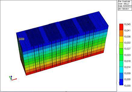
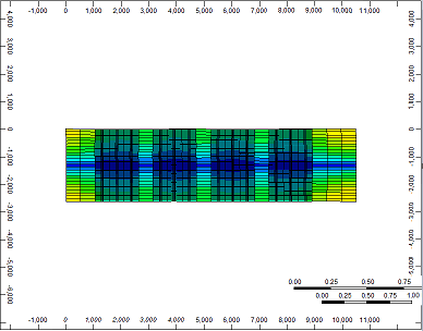
1 1 = A tight oil reservoir of 20 ft × 20 ft × 10 ft Grid cells dimension was built. The average matrix permeability of the reservoir is 0.7 ×10⁻² mD and average porosity 5.6 %. The average thickness of the reservoir is 5ft. Formation oil density is 600 kg/𝑚3 and formation oil viscosity is 1.2 mPa.s. The GOR is 60. 𝑚𝑚. The formation pressure is 12 MPa and the crude oil volume factor is 1.127. Figure 3 presents the reservoir model including 4 fracturing stages for the Bakken tight oil reservoir. Three effective fractures per stage.
cig kigw ciw $$ \sum_ {k = 1} ^ {n} c _ {i o} = 1 $$
= $$ \sum_ {k = 1} ^ {n} c _ {i w} = 1 $$
𝑆𝑜 + 𝑆𝑤 + 𝑆𝑔= 1
𝑃𝑐𝑜𝑤= 𝑃𝑜 − 𝑃𝑤
𝑃𝑐𝑔𝑜= 𝑃𝑔 − 𝑃𝑜
Reservoir Characteristics and Numerical Simulation Model
Reservoir Description
parameters during history matching are listed in Table 1. Furthermore, some relative permeability curves such as water-oil relative permeability and liquid-gas relative permeability were obtained by tuning them to fit a good history matching as shown in Figure 7.

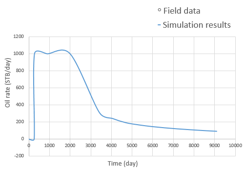
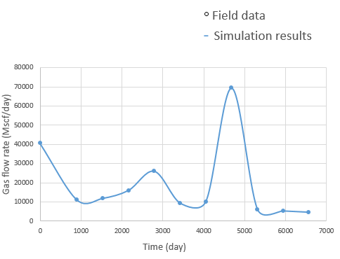
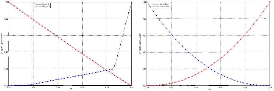
Water-oil relative permeability curve Liquid-gas relative permeability curve Figure 7: Relative permeability curves for a good history matching.
| Parameter | Value | Unit | ||||||
|---|---|---|---|---|---|---|---|---|
| The model dimensions | 10500 ×2640 ×50 | ft | ||||||
| Initial reservoir temperature | 7800 | Psi | ||||||
| Production time | 1.2 | Year | ||||||
| Reservoir temperature | 245 | ℉ | ||||||
| Initial water saturation | 0.41 | Value | ||||||
| Total compressibility | 1 × 10⁻⁶ | 𝑝𝑠𝑖−1 | ||||||
| Matrix permeability | 5 | μD | ||||||
| Matrix porosity | 0.056 | Value | ||||||
| Horizontal well length | 8828 | ft | ||||||
| Number of stages | 15 | Value | ||||||
| Total number of fractures | 60 | Value | ||||||
| Fracture conductivity | 50 | mD-ft | ||||||
| Fracture half-length | 215 | ft | ||||||
| Fracture height | 50 | ft |
Table 1: Parameters used for history matching (Bakken formation).
Based on a tight oil reservoir, a simulation model of CO2 huff-n-puff process in a horizontal well with multi- stage fractures is built. In this work, we first of all started by producing for four years and then the horizontal well is converted to CO2 injector with injection rates of 100 MSCF/day. After six months of injection, the well is shut- in and soaking for three months. Finally, the well is put back in production for one year. This represents one cycle of CO2 huff-n-puff. The cycle will start again at the end of the year of production and will cover the 30 years.
Many cases are studied in this simulation to investigate the sensitivity study. For the base case, we set up one fracture per stage for a total of 4 stages. For each stage fracture width is 0.03 ft, fracture half-length is 1300
- 𝐶−𝐶 𝐶−𝐶30, and their corresponding molar fractions are 0.01%, 22.03%, 11.67%, 28.15%, 9.4% and 8.08%, respectively. Table 3 presents the order detailed input
- Component
- Molar
- Fracture
- Critical Pressure
- Critical
- Temperature (k)
- Critical Volume (atm)
- (L/mol)
- Factor
- CO2
- 0.0001
- 72.8
- 304.2
- 0.094
- 44.01
- 0.225
- 𝑁2-𝐶1
- 0.2203
- 45.24
- 189.67
- 0.0989
- 16.21
- 0.0084
- 𝐶1-𝐶4
- 0.2063
- 43.49
- 412.47
- 0.2039
- 44.79
- 0.1481
- 𝐶5-𝐶7
- 0.117
- 37.69
- 556.92
- 0.3324
- 83.46
- 0.2486
- 𝐶8-𝐶12
- 0.2815
- 31.04
- 667.52
- 0.4559
- 120.52
- 0.3279
- 𝐶13- 𝐶19
- 0.094
- 19.29
- 673.76
- 7649
- 220.34
- 0.5672
- 𝐶20-𝐶30
- 0.0808
- 15.38
- 792.4
- 1.2521
- 321.52
- 0.9422
Table 2: Compositional data for the Peng-Robinson EOS in Bakken.
| Parameter | Value | Unit | ||||||
|---|---|---|---|---|---|---|---|---|
| The model dimensions | 20 ×20 ×10 | ft | ||||||
| Initial reservoir temperature | 7800 | Psi | ||||||
| Production time | 30 | Year | ||||||
| Reservoir temperature | 240 | ℉ | ||||||
| Initial water saturation | 0.2 | Value | ||||||
| Total compressibility | 1 × 10⁻⁶ | 𝑝𝑠𝑖−1 | ||||||
| Matrix permeability | 0.007 | μD | ||||||
| Matrix porosity | 0.056 | Value | ||||||
| Horizontal well length | 8828 | ft | ||||||
| Number of stages | 4 | Value | ||||||
| Total number of fractures | 12 | Value | ||||||
| Fracture conductivity | 6.9 | mD-ft | ||||||
| Fracture half-length | 1300 | ft | ||||||
| Fracture height | 10 | ft |
Table 3: Compositional data for the Peng-Robinson EOS in Bakken.
Results and Discussions
As mentioned above, eight uncertain parameters (as listed in Table 4) were studied to analyze the sensitivity of CO2 huff-n-puff process in the Bakken tight oil. The effect
| Parameter | Value 2 | Base case | Value 3 | ||||||||
|---|---|---|---|---|---|---|---|---|---|---|---|
| Number of fracture | 1 | 2 | 3 | ||||||||
| CO injection rate, Mscf/day 2 | 50 | 100 | 500 | ||||||||
| CO injection time, month 2 | 3 | 6 | 9 | ||||||||
| Number of cycle | 3 | 17 | 10 | ||||||||
| CO soaking time, month 2 | 5 | 3 | 6 | ||||||||
| Fracture permeability, mD | 500 | 230 | 800 | ||||||||
| Fracture half-length, ft | 650 | 1300 | 2000 | ||||||||
| Reservoir permeability, mD | 0.003 | 0.007 | 0.01 |
Table 4: Eight parameters used for sensitivity study.
Effect of Number of Fracture per Stage on Oil Recovery Factor
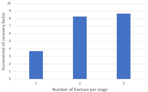
For this case, we successively set up 1, 2, and 3 fractures per stage; while keeping the other parameters the same as those in the base case. We obtained an oil recovery factor of 8.3%, 8.56%, and 8.67% respectively as shown in Figure 9. It can be seen that the oil recovery increases with an increase of the number of fracture per stage.
Effect of CO2 Injection Rate on oil Recovery
Factor
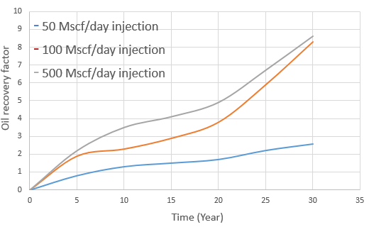
For this case, we successively set up CO2 injection rate to be 50 Mscf/day, 100 Mscf/day, and 500 Mscf/day; while keeping the other parameters the same as those in the base case. We obtained an oil recovery factor of 2.56%, 8.3%, and 8.6% respectively as shown in Figure 10. It can be seen that the oil recovery increases with an increase of CO2 injection rate.
Effect of CO2 Injection Time on Oil Recovery
Factor
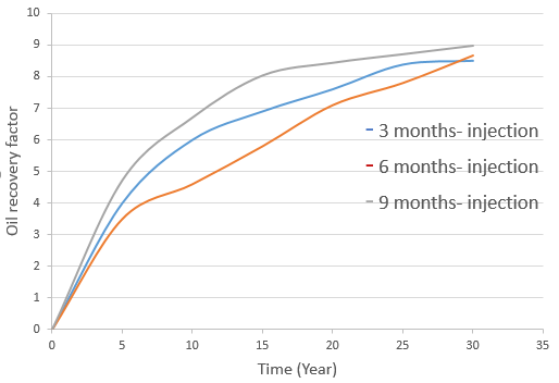
For this case, we successively set up CO2 injection time
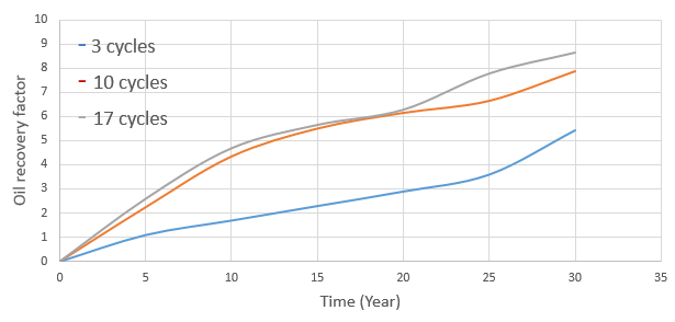
Effect of Number of CO2 Huff-N-Puff Cycle on Oil Recovery Factor
For this case, we successively set up the number of cycle to be 3, 10, and 17; while keeping the other parameters the same as those in the base case. We obtained an oil recovery factor of 5.43%, 7.9%, and 8.67% respectively as shown in Figure 12. It can be seen that the oil recovery increases with the increase of the number of CO2 huff-n-puff cycle.
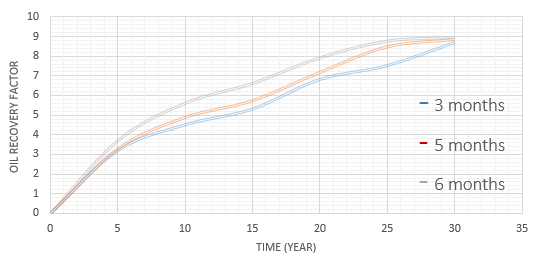
Effect of CO2 Soaking Time on Oil Recovery
Factor
For this case, we successively set up CO2 soaking time to be 3 months, 5 months, and 6 months; while keeping the other parameters the same as those in the base case.
We obtained an oil recovery factor of 8.67%, 8.87%, and 8.93% respectively as shown in Figure 13. It can be seen that the oil recovery increases with the increase of the soaking time.
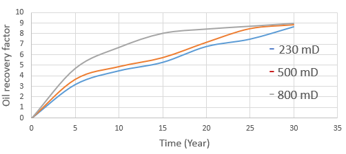
Effect of Fracture Permeability on Oil Recovery Factor
For this case, we successively set up the fracture permeability to be 230 mD, 500 mD, and 800 mD; while keeping the other parameters the same as those in the base case. We obtained an oil recovery factor of 8.67%, 8.87%, and 8.97% respectively as shown in Figure 14. It can be seen that the oil recovery increases with the increase of the fracture permeability.
$$ = \frac {A K \Delta P}{\mu L} (1) $$
AK P q L μ
Darcy’s law: D
3 $$ = \frac {w e ^ {3} \Delta p}{1 2 \mu L} (2) $$
we p q L μ Poiseuille’s law:
12 p
3 $$ \frac {A K \Delta P}{\mu L} = \frac {w e ^ {3} \Delta p}{1 2 \mu L} $$
Combining 1 and 2 we get
3 we K=
k is the intrinsic fracture permeability.
12 A From the equations we can deduce that the flow rate increases with the increase of fracture permeability; that is why this parameter is really important when studying CO2 injection in tight oil reservoirs.
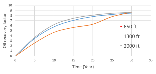
Effect of Fracture Half-Length on Oil Recovery Factor
For this case, we successively set up the fracture half- length to be 650 ft, 1300 ft, and 2000 ft; while keeping the other parameters the same as those in the base case. We obtained an oil recovery factor of 8.5%, 8.67%, and 8.7% respectively as shown in Figure 15. It can be seen that the oil recovery increases with the increase of the fracture half-length.
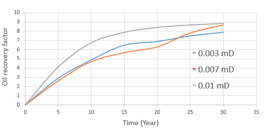
Effect of Reservoir Permeability on Oil
Recovery Factor
For this case, we successively set up the reservoir permeability to be 0.003 mD, 0.007 mD, and 0.01 mD;
while keeping the other parameters the same as those in the base case. We obtained an oil recovery factor of 7.9%, 8.67%, and 8.86% respectively as shown in Figure 16. It can be seen that the oil recovery increases with the increase of reservoir permeability.
Summary and Conclusions
After performing a series of simulations for the CO2 huff-n-puff process for enhanced oil recovery in the Bakken formation, the following conclusions can be drawn: 1. The relative permeability curves, such as water-oil relative permeability and liquid-gas relative permeability are obtained based on history matching with a fractured well from the Middle Bakken. 2. The case with three effective hydraulic fractures within one perforation stage has the highest incremental oil recovery factor compared to the other cases with one and two fractures within one perforation stage.
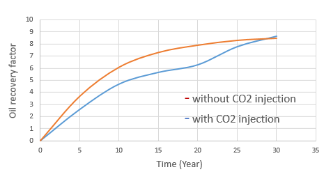
3. A comparison of the oil recovery factor with and without gas injection has proved that it is higher when injecting gas (Figure 17). 4. CO2 molecular diffusivity is a significant factor in the reservoir simulation model to capture the real physics mechanism during CO2 injection into the tight oil reservoirs 5. Oil recovery factor increases with the increasing number of cycle of CO2 huff-n-puff, number of fracture per stage, CO2 injection time, CO2 injection rate, CO2 soaking time, fracture permeability; fracture conductivity and reservoir permeability. 6. The range for the incremental oil recovery factor at 30 years of production is obtained as 2.56% - 8.97%.
Acknowledgment
I would first of all like to acknowledge the National Natural Science Foundation of China under Grant no. 51574265 for the financial support of this work. I would also thank China University of Petroleum (East China) for the assistance during the realization of this work and Computer Modeling Group Ltd. for providing the CMG- GEM software.
Nomenclature
Nomenclature bbl = barrels MMP = Minimum miscibility pressure, psi CMG = Computer Modeling Group GOR = Gas oil ratio Mscf = 103 standard cubic feet, 𝑓𝑡3 mD = 103 Darcy
References
-
West DRM, Harkrider J, Besler MR, Barham M, Mahrer KD (2013) Optimized production in the Bakken shale: south Antelope case study. SPE Unconventional Resources Conference, Society of Petroleum Engineers, Calgary, Canada.
-
Iwere FO, Heim RN, Cherian BV (2012) Numerical simulation of enhanced oil recovery in the middle Bakken and upper Three Forks tight oil reservoirs of the Williston basin. SPE Americas Unconventional Resources Conference, Society of Petroleum Engineers, Pittsburgh, Pennsylvania, USA.
-
Pilcher RS, Ciosek JM, McArthur K, Hohman J, Schmitz PJ (2012) Ranking Production Potential Based on key Geological Drivers-Bakken Case Study. International Petroleum Technology Conference, International Petroleum Technology Conference, Bangkok, Thailand.
-
United States Geological Survey 2013.
-
Ganpule S, Cherian B, Gonzales V, Hudgens P, Aguirre PR, et al. (2013) Impact of well completion on the uncertainty in technically recoverable resource estimation in Bakken and Three Forks. SPE Unconventional Resource Conference, Society of Petroleum Engineers, Calgary, Canada.
-
Flowers JR, Guetta DR, Stephenson CJ, Jeremie P, d'Arco N (2014) A statistical study of proppant type vs. well performance in the Bakken central basin. SPE Hydraulic Fracturing Technology Conference, Society of Petroleum Engineers, The Woodlands, Texas, USA.
-
Handren P, Palisch T (2007) Successful hybrid slickwater fracture design evolution-an east Texas cotton valley taylor case history. SPE Annual Technical Conference and Exhibition, Society of Petroleum Engineers, Anaheim, California, USA.
-
Zhou X, Yuan Q, Zhang Y, Zhang L (2019).
-
Yu W, Lashgari HR, Sepehrnoori K, The University of Texas at Austin.
-
Arshad A, Al-Majed A, Maneouar H, Muhammadain A, Mtawaa Pl.
- Nigeria’s Vulnerability in the Face of Global Energy Policy
- A Simulation Study of Investigation of Optimum Oil Production Performance by Applying Various Gas Injection Methods in Oil Reservoir
- Characterization of Permo-Triassic Reservoirs through Thermal Maturity Assessment of Westphalian Source Rocks in the Cheshire Basin
- Influence of Microwax on the Rheological and Thermal Behaviour of a Wax Crude Oil
- Real-Time Monitoring and Performance Optimization of Steam Injection in Heavy Oil Reservoirs Using Fiber Optic Sensing and Integrated Predictive Simulation Models
- Rapid On-Site Determination of the Total Petroleum Hydrocarbon Content of Soils by Handheld Fourier Transform Near-Infrared Spectroscopy: Development of a Global, Site- and Scanner- Independent Calibration Model