A Machine Learning Approach to Modeling Pore Pressure
Machine Learning techniques and applications have lately gained a lot of interest in many areas, including spheres of arithmetic, finances, engineering, dialectology, and a lot more. This is owing to the upwelling of ground-breaking and sophisticated machine learning procedures to exceedingly multifaceted complications along with the prevailing advances in high speed computing. Numerous usages of Machine learning in daily life include pattern recognition, automation, data processing and analysis, and so on. The Petroleum industry is not lagging behind also. On the contrary, machine learning approaches have lately been applied to enhance production, forecast recoverable hydrocarbons, augment well placement by means of pattern recognition, optimize hydraulic fracture design, and to help in reservoir characterization. In this paper, three different machine learning models were trained and utilized to explore the feasibility of forecasting pore pressure of a well. The machine learning algorithms include, Simple Linear Regression, Decision Stump and Multilayer Perceptron (ANN). The predictive accuracies of the algorithm was analyzed using statistical measures. Five (5) parameters were utilized as input variables in the models: hydrostatic pressure, overburden pressure, observed and normal sonic velocities and pore pressure. 80% of the data was used in training while the remaining 20% was used for testing of the models. A sensitivity analysis of the five variable was conducted so as to identify correlations of the variables. Results of the sensitivity analysis revealed that both hydrostatic and overburden pressures appear to have the strongest correlation with pore pressure (0.766) and closely followed by normal compacted sonic velocity (0.753). Meanwhile, observed sonic velocity has the least correlation (0.046). The models were appraised by determining their Relative Absolute Errors. Results indicate that Multilayer Perceptron has the best prediction and least Relative Absolute Error of 5.77%. While the Decision Stump model had a Relative absolute error of 54.41%. The Simple Linear Regression had a relative absolute error of 67.93%. By and large, all three models appear to be suitable for modeling pore pressure but the Multilayer Perceptron is the most accurate.
Introduction
Machine learning models are nowadays essential and commonly useful means for forecasting vital variables for complex oil and gas systems with numerous influencing variables displaying highly irregular and/or non-linear relationships. Their application and diversity are growing by Schmidhuber J [1]. Machine learning methods have caught the eyes of engineers thanks to their ability to associate input data to the output data.
Machine learning methods were utilized expansively in the majority of petroleum engineering purposes, such as, drilling, reservoir, production and engineering, as well as petrophysics, rock mechanics and exploration [2]. One of such is the Response Surface Model which is utilized in numerous facets of reservoir engineering such as history matching [3, 4], determining the initial uncertainty of hydrocarbons [5], locating spots for well placement [6] and estimating initial hydrocarbon uncertainty. Production variation has been forecasted with the aid of pattern recognition based on the well locations. Mohaghegh SD, El-Sebakhy E introduced a novel computational intelligence modeling plan founded on the support vector machines SVR system to forecast both bubble point pressure and oil formation volume factor [7, 8, 9, 10]. They utilized solution gas-oil ratio, reservoir temperature, oil gravity, and gas relative density as input parameters. Oloso (2009) established two novel models for assessing the viscosity and solution gas/oil ratio (GOR) [11].
Artificial Neural Networks are computational techniques that mimics the human brain in unraveling solutions to problems. It consists of a series of interconnected nodes, which are more or less the artificial versions of the neurons in the brain. Each node symbolizes the artificial neuron, while the arrows symbolize the link from an output node to an input node.
Usually, the most common methods used to predict formation pressure prior to drilling is by using correlations that require well logs or seismic analysis data as input parameters. However, these correlations have their limitations in that they are based on limited data sets that are not readily available, thus making such predictions somewhat tedious. Consequently, the oil and gas industry is constantly seeking for alternative techniques of forecasting pore pressures that are not so dependent on well log data. It is on this account that we adopt and assess the machine learning approach so as to ascertain their suitability to formation pressure prognosis.
Simple Linear Regression
The model learns a linear regression model based on a single attribute, it chooses the attribute that yields the least square error. It can deal with numeric attributes.
Multiple Layer Perceptron
This is a neural network that is trained using back propagation to learn to predict instances. This network has three layers: an input layer on the left with one rectangular box for each attribute (colored green); a hidden layer next to it (red) to which all the input nodes are connected; and an output layer at the right (orange). The labels at the far right show the classes that the output nodes represent. Output nodes for numeric classes are automatically converted to unthresholded linear units.
Decision Stump
It does regression based on mean-squared error or classification based on entropy. It is designed for use with the boosting methods, builds one-level binary decision trees for datasets with a categorical or numeric class, dealing with missing values by treating them as a separate value and extending a third branch from the stump. Usually used in conjunction with a boosting algorithm.
Methodology
The methodology implemented for the work involved using 80% of the actual pore pressure data in training the three models while the remaining 20% was used for testing of the models. A sensitivity analysis was carried out in this work using scatter plots. This involved plotting the variables (hydrostatic pressure, lithostatic pressure, observed sonic compressional velocity Vp, and normal compacted shale velocity Vn) against one another. These plots give a very vivid and simplified illustration of the variables’ sensitivity. The strength of the correlations between the variables was computed using the linear correlation coefficient [12].
− − − − ∑ x x y y i i s s x y r n ( )( )
(1) = −
1 − x = sample mean of the predictor variable Where
xs = standard deviation of the predictor variable −y = sample mean of the response variable xy = standard deviation of the response variable n=sample size
Performance of Models
A statistical measure was applied to ascertain the predictive accuracies of the algorithms. The measure was the Relative Absolute Error.
Results and Discussion
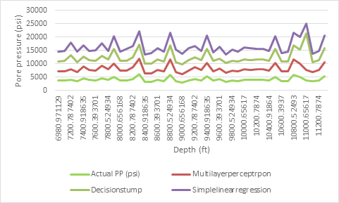
The outcome of the pore pressure modeling are presented below. Results reveal that the Multilayer Perceptron (ANN) accurately predicted pore pressure across most instances. This is evidenced by the low Relative absolute error of
5.77%. The decision stump also yielded good predictions with Relative absolute error of 54.41%. The simple linear regression model yielded the least accuracy of the three models with a Relative Absolute Error of 67.93% (Table 1-2).
| Actual PP (psi) | Multilayer Perceptrpon | Error | Decision Stump | Error | Simple Linear Regression | Error |
|---|---|---|---|---|---|---|
| 3594.011 | 3568.511 | -25.5 | 3700.757 | 106.747 | 3592.914 | -1.096 |
| 3646.879 | 3619.062 | -27.817 | 3700.757 | 53.878 | 3768.246 | 121.367 |
| 3978.16 | 3931.212 | -46.948 | 5302.041 | 1323.88 | 4624.097 | 645.937 |
| 3396.181 | 3367.373 | -28.808 | 3700.757 | 304.577 | 3947.288 | 551.107 |
| 4478.573 | 4492.593 | 14.02 | 3700.757 | -777.816 | 4216.355 | -262.218 |
| 3884.521 | 3889.688 | 5.166 | 3707.041 | -177.481 | 3359.318 | -525.204 |
| 3693.725 | 3668.527 | -25.198 | 3707.041 | 13.315 | 3937.371 | 243.646 |
| 4635.664 | 4609.2 | -26.464 | 3707.041 | -928.623 | 4626.092 | -9.573 |
| 3912.968 | 3923.552 | 10.584 | 3707.041 | -205.928 | 3316.009 | -596.959 |
| 5077.577 | 5078.88 | 1.304 | 5429.303 | 351.727 | 4671.212 | -406.365 |
| 3666.297 | 3665.683 | -0.614 | 3716.706 | 50.409 | 3504.419 | -161.878 |
| 3697.584 | 3692.041 | -5.543 | 3716.706 | 19.122 | 4419.735 | 722.151 |
| 4341.272 | 4371.699 | 30.426 | 3716.706 | -624.567 | 4208.815 | -132.458 |
| 5990.89 | 5933.745 | -57.146 | 5215.934 | -774.956 | 4895.377 | -1095.51 |
| 3193.493 | +3217.351 | 23.857 | 3716.706 | 523.212 | 3225.24 | 31.747 |
| 3093.845 | 3130.836 | 36.991 | 3747.078 | 653.232 | 3925.674 | 831.829 |
| 3916.394 | 3875.2 | -41.195 | 3747.078 | -169.316 | 4356.151 | 439.757 |
| 3558.819 | 3482.809 | -76.01 | 3747.078 | 188.258 | 3838.111 | 279.292 |
| 5764.953 | 5766.679 | 1.726 | 5244.176 | -520.777 | 4933.404 | -831.549 |
| 3388.047 | 3510.594 | 122.547 | 3747.078 | 359.031 | 4533.01 | 1144.963 |
| 3027.477 | 3059.142 | 31.665 | 3716.499 | 689.022 | 3854.903 | 827.426 |
| 3733.722 | 3779.288 | 45.567 | 3716.499 | -17.223 | 4588.498 | 854.776 |
| 4357.154 | 4322.766 | -34.389 | 3716.499 | -640.655 | 4175.159 | -181.995 |
| 3786.709 | 3803.458 | 16.749 | 3716.499 | -70.21 | 3458.754 | -327.955 |
| 5184.277 | 5184.914 | 0.637 | 5316.761 | 132.483 | 4815.115 | -369.162 |
| 3618.611 | 3632.898 | 14.287 | 3722.596 | 103.985 | 3254.789 | -363.822 |
| 4116.115 | 4113.96 | -2.155 | 3722.596 | -393.519 | 4354.416 | 238.301 |
| 3258.714 | 3309.186 | 50.471 | 3722.596 | 463.882 | 3073.216 | -185.498 |
| 3723.978 | 3693.664 | -30.314 | 3708.781 | -15.197 | 4042.469 | 318.492 |
| 3575.72 | 3518.66 | -57.06 | 3708.781 | 133.061 | 3641.539 | 65.819 |
| 3976.176 | 3967.18 | -8.996 | 3708.781 | -267.395 | 4309.866 | 333.69 |
| 3868.439 | 3880.146 | 11.706 | 3708.781 | -159.658 | 4445.456 | 577.017 |
| 3955.665 | 3910.463 | -45.203 | 3704.245 | -251.421 | 4054.808 | 99.143 |
| 3926.871 | 3885.181 | -41.689 | 3704.245 | -222.626 | 4097.6 | 170.729 |
| 3698.16 | 3655.713 | -42.447 | 3704.245 | 6.085 | 3667.494 | -30.666 |
| 5104.135 | 5137.625 | 33.49 | 5326.779 | 222.643 | 4756.179 | -347.957 |
| 3517.212 | 3617.109 | 99.897 | 3727.812 | 210.6 | 3252.878 | -264.334 |
| 3581.517 | 3595.871 | 14.354 | 3727.812 | 146.295 | 3529.754 | -51.763 |
| 5775.789 | 5716.045 | -59.745 | 5284.118 | -491.672 | 4919.433 | -856.357 |
| 4953.752 | 4974.705 | 20.953 | 5284.118 | 330.366 | 4789.31 | -164.442 |
| 3798.472 | 3763.202 | -35.27 | 13723.844 | -74.628 | 3667.966 | -130.506 |
| 3357.758 | 3414.65 | 56.892 | 3723.844 | 366.086 | 3105.226 | -252.532 |
| 3797.28 | 3875.678 | 78.399 | 3723.844 | -73.435 | 3278.843 | -518.437 |
| 5231.326 | 5243.386 | 12.06 | 5310.88 | 79.554 | 4706.971 | -524.355 |
Table 1: Table presenting results of pore pressure modelling using the three models.
| Decision Stump | Simple Linear Regression | Multilayer Perceptron | |
|---|---|---|---|
| Relative absolute error | 54.41% | 67.93% | 5.77% |
Table 2: Statistical Performance of the models.
Sensitivity Analysis
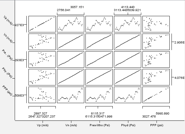
The cross-plots of hydrostatic pressure, overburden pressure and sonic velocities against the measured pore pressure above showed varying degrees of correlation with the pore pressure. The cross-plot of normal compacted shale sonic compressional velocity (Vn) against pore pressure (bottom left) showed that sonic compressional velocity has a strong influence on the pore pressure as both parameters increased together and are tightly positioned along an imaginary line thereby implying a positive correlation. The scatter plot of observed sonic velocity (Vp) and pore pressure (top right) initially showed a positive correlation but later exhibited a negative correlation (decrease of Vp with increase in pore pressure). More so, the data points where spread out around the imaginary line, implying the correlation is not very strong. Lastly both the hydrostatic and overburden pressures showed strong correlations with the measured pore pressure as they both increase with it. Furthermore, results of the computed correlation measure of the input variables and the pore pressure shows that the hydrostatic pressure (0.766), overburden pressure (0.766) and normal compacted sonic velocity (0.75) have strong correlations with the pore pressure as their values are close to 1. The observed sonic velocity however, appears to have a weak relationship with pore pressure as it yielded a value of 0.47 which is quite far from 1 (Figure 1).
Overall it can be surmised that all model input parameters are crucial to the pore pressure predictions of the model but the parameters with the most effect on the pore pressure predictions appear to be the hydrostatic and overburden pressures as well as the normal compacted sonic velocity (Vn) owing to their positive correlations with the pore pressure (Figure 2).
Confusion Matrix
| Row Id | Vp (m/s) | Vn (m/s) | Pres Litho (psi) | Phyd (psi) | PPP (psi) |
|---|---|---|---|---|---|
| Vp (m/s) | 1 | 0.6903 | 0.6747 | 0.6817 | 0.04642 |
| Vn (m/s) | 0.6903 | 1 | 0.9992 | 0.9996 | 0.75292 |
| Pres-Litho (psi) | 0.6747 | 0.9992 | 1 | 0.9999 | 0.7658 |
| Phyd (psi) | 0.6817 | 0.9996 | 0.9999 | 1 | 0.7600 |
| PPP (psi) | 0.04642 | 0.7529 | 0.7658 | 0.7600 | 1 |
Table 3: Values of the confusion matrix.
Conclusion
Machine Learning algorithms can be realistically trained and utilized to direct pressure measurements in other to forecast pore pressure. In this work, the pore pressure of a formation was predicted using existing pore pressure data with the aid of three machine learning models namely, Simple Linear Regression, Decision Stump and Multilayer Perceptron. The models were trained with Eighty percent of the dataset after which the remaining twenty percent was utilized in the validation of the models’ accuracies. Results obtained showed that the Multilayer Perceptron model has a laudable prediction accuracy. The Decision Stump model equally showed a good prediction performance. The Simple Linear Regression had the highest Relative Absolute Error. Furthermore, sensitivity analysis of the data used in the work showed that the hydrostatic pressure, overburden pressure and normal compacted sonic velocity have best correlations with the pore pressure as their values are closest to 1. On the whole, it can be surmised that the Multilayer Perceptron can be successfully utilized in the projection of pore pressures as demonstrated by the end result.
References
-
Schmidhuber J (2015) Deep Learning in Neural networks: An Overview. Neural Networks 61: 85-117.
-
Anifowose FA, Ewenla AO, Eludiora SI (2011) Prediction of Oil and Gas Reservoir Properties Using Support Vector Machines. International Petroleum Technology Conference, Bangkok.
-
Ahmadi MA, Ebadi M, Hosseini SM (2014) Prediction breakthrough time of water coning in the fractured reservoirs by implementing low parameter support vector machine approach. Fuel 117(Part A): 579-589.
-
Ahmadi MA, Ebadi M, Shokrollahi A, JavadMajidi SM (2013) Evolving artificial neural network and imperialist competitive algorithm for prediction oil flow rate of the reservoir. Applied Soft Computing 13(2): 1085-1098.
-
Mohaghegh S (2006) Quantifying uncertainties associated with reservoir simulation. SPE Annual Technical Conference and Exhibition, USA.
-
Ahmadi MA, Soleimani R, Alireza B (2014) A Computational Intelligence Scheme for prediction of equilibrium water dew point of natural gas in TEG dehydration systems. Fuel 137: 145-154.
-
Manceau E, Mezghani M, Zabalza-Mezghani I, Roggero F (2001) Combination of experimental design and joint modeling methods for quantifying the risk associated with deterministic and stochastic uncertainties. SPE Annual Technical Conference and Exhibition, Louisiana.
-
Mohaghegh S, Arefi R, Ameri S, Hefner MH (1994) A methodological approach for reservoir heterogeneity characterization using artificial neural networks. SPE Annual Technical Conference and Exhibition, Louisiana.
-
Mohaghegh SD, Liu JS, Gaskari R, Maysami M, Olukoko OA (2012) Application of well based surrogate reservoir models (SRMs) to two offshore fields in Saudi Arabia. SPE Western Regional Meeting, USA.
-
El-Sebakhy E, Sheltami T, Shaaban Y, Raharja PD (2007) support vector machines framework for predicting the PVT properties of crude oil systems. SPE Middle East Oil & Gas show and conference, Bahrain.
-
Oloso M, Khoukhi A, Abdulraheem A (2009) Prediction of crude oil viscosity and gas/oil ratio curves using recent advances to neural networks. SPE/EAGE Reservoir Characterization and Simulation Conference, UAE.
-
ThoughtCo (2019) Calculating the Correlation Coefficient.
-
Ian Witten, M. H. (2016). Data Mining. Morgan Kaufmann.
- Nigeria’s Vulnerability in the Face of Global Energy Policy
- A Simulation Study of Investigation of Optimum Oil Production Performance by Applying Various Gas Injection Methods in Oil Reservoir
- Characterization of Permo-Triassic Reservoirs through Thermal Maturity Assessment of Westphalian Source Rocks in the Cheshire Basin
- Influence of Microwax on the Rheological and Thermal Behaviour of a Wax Crude Oil
- Real-Time Monitoring and Performance Optimization of Steam Injection in Heavy Oil Reservoirs Using Fiber Optic Sensing and Integrated Predictive Simulation Models
- Rapid On-Site Determination of the Total Petroleum Hydrocarbon Content of Soils by Handheld Fourier Transform Near-Infrared Spectroscopy: Development of a Global, Site- and Scanner- Independent Calibration Model