Econometric Perspective of the Oil Consumption and Economic Growth Relation in India
This research aims to study the existence and direction of the short-run or long-run relationship between per capita oil consumption and gross domestic product in India. The data from 1965 to 2015 had analyzed by employing the vector error correction model. For the verification of the same result, a standard Granger causality test had performed. The study results have suggested the existence of a long-run relationship and show the direction of changes in gross domestic product cause changes in oil consumption. As a policy implication, economic growth can be considered a policy variable to improve India's oil resources.
Introduction
Over the past two decades, the rapid growth of the Indian economy has reflected its growing demand for petroleum products. As of 2018, India was the world’s third- largest user of 5.2 million barrels of oil per day, exceeded only by the world’s two largest economies, the US and China. Consumption has risen almost 1.7 times since 2008 and has exceeded the figures for Japan. India also reported more substantial growth than China post-2010, particularly between 2015 and 2016, when consumption increased by 8 per cent-10 percent per year [1, 2]. India expected to overtake China in terms of oil consumption by the mid-2020s. Table 1 shows the production and consumption of oil per capita in India.
At the same time, the massive demand for commodities in India can hardly satisfy domestic oil production. Oil production in the last decade, between 35 and 37mn tonnes per year, was relatively constant. In addition to the adverse effects of geopolitical instability and volatile petroleum Policy Article prices, the production of Indian oil by 2024 could increase significantly. However, recent data show that crude oil production otherwise decreased continuously since 2012 and declined to 34.2 million tonnes in 2019, the lowest amount since 2010 [1, 2]. The aging of petroleum fields in the country hampers crude oil production. India’s territory also makes it difficult for oil and gas to explore, and the requisite skills exceed the abilities of local government companies. The usual assumption is that it is an electric source or a diesel source for vehicles concerning the use of petroleum. Petroleum products have a much wider variety of uses for the manufacture in almost every kind of daily life of asphalt, highway gasoline, various plastics, chemical, and synthetic materials. There is no distinction in this regard for India, fuel like gasoline, engine spirits, and turbine aviation, used commonly in petroleum products: bitumen (used for road building), grades and lubricants, and oil coke. However, fuel is still the bulk of oil consumption, with 39.1 percent of total oil consumption dropping into high-speed diesel and the engine’s spirit (14.2 percent) and liquified fuel gas (12.2 percent).
| Year | Oil Production | Oil Consumption |
|---|---|---|
| 2005 | 353.359 | 1239.12 |
| 2006 | 359.097 | 1283.69 |
| 2007 | 357.604 | 1360.99 |
| 2008 | 365.479 | 1405.68 |
| 2009 | 362.313 | 1461.22 |
| 2010 | 388.235 | 1468.09 |
| 2011 | 398.219 | 1520.09 |
| 2012 | 390.303 | 1598.24 |
| 2013 | 385.006 | 1594.97 |
| 2014 | 373.18 | 1625.55 |
| 2015 | 364.884 | 1739.88 |
Table 1: Oil production and oil consumption in India.
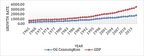
Due to its value in all life aspects, it is not surprising that economists consider their consumption as a useful economic measure of success. As a leading indicator, oil consumption and GDP now have templates for developed and developing economies. Indian data shows that a similar decline in petroleum consumption occurred at the start of the GDP growth deceleration in Q1 2018. Figure 1 shows the growth pattern between oil and gross domestic product in India.
India’s strategy for tackling its overreliance on oil imports is mainly based on two actions to promote domestic development and the focus on renewable energy sources. In its oil consumption policies, the Indian government had more than helped, enabling up to 100 percent FDI in many petroleum and gas sectors. The program had designed to promote exploration and development of petroleum and natural gas and decrease dependence on imports, such as HELP (hydrocarbon Exploration and Licensing Policy) and OALP (Open Acreage Licensing Program).
So, looking at the importance of oil consumption in economic development, this research paper has attempted to analyze the interaction between oil production and India’s gross domestic product. The study’s core problem discussed in this section is the second section, Data, and Methodology, followed by the third section, Results, and Discussion. Based on the given results, the Conclusion and some Policy Implications had suggested in the last section.
Data and Methodology
Data
To find the relationship between per capita oil consumption and per capita gross domestic product in India, the annual data took for 1965-66 to 2015-16 (the latest available). The data of per capita oil consumption and per capita gross domestic product (Constant 2010 US$) from www.data.worldbank.org. A three-stage procedure was employed to know the relationship, and the study results had calculated with the help of statistical application EViews (IHS Global Inc., USA).
Unit Root Test
As a first step, Augmented Dickey-Fuller (ADF) performed to know the stationarity of time series data and a null hypothesis set, i.e., series is non-stationary [3]. So, the following intercept took into consideration:
1 Y OC oc t t t α α µ ∆ = + + (1)
Where Yt , OCt and t µ are Gross Domestic Product, Oil Consumption and t µ the error term.
Johansen Co-Integration
Co-Integration test helps in verifying the null hypothesis : int 0 H Thereis noco egration − [4]. The two parameters of the Johansen co-integration tests are the Trace test and maximum eigenvalue test.
n LR r n T In i i ro λ = − − ∑ = +
( ) ( ) 0, 1 1
(2) ( ) ( ) 0 0 0 1 ln 1 1 LR r r T r λ + + = − + (3)
Vector Error Correction Model (VECM)
As the third stage will enable exploring both the short
Results and Discussions
and long-run dynamics of co-integrated sequence [5]. The conventional ECM for co-integrated series is:
n n LOC LOC LGDP z o t t i t i i t i t i i α α δ ϕ µ ∆ = + ∆ + ∆ + + ∑ ∑ − − − = =
1 1 0 (4) n n LGDP LGDP LOC z t t i t i i t i t i i β β δ ϕ µ ∆ = + ∆ + ∆ + + ∑ ∑ − − − = =
0 1 1 0 (5) Where, z is the ECT (Error Correction Term), and it is the OLS (Ordinary Least Square) residual from the following long- run co-integrating regression: 1 LOC LGDP o t t t α α µ = + + and 0 1 LGDP LGDP t t t β β µ = + + are defined as
1 1 1 1 1 z ECT LOC LGDP o t t t t α α = = − − − − − −. To verify the results of VECM, a standard Granger Causality Test is also employed, which validates the direction of causality flow from one to the other variables and vice versa [6]. The model of the Granger causality test is as follows:
k k LOC LOC LGDP t i t i i t i i i α β γ µ ∆ = + ∆ + ∆ + ∑ ∑ − − = =
(6)
1 1 k k LGDP LGDP LOC t i t i i t i i i α β ψ µ ∆ = + ∆ + ∆ + ∑ ∑ − − = =
(7)
1 1 Whereasα , β , ψ , and γ are parameters to be estimated and µ represent the serial error terms, LOCt and LGDPt are defined observation for the t periods; ∆is the differential operator; k refers to the number of lags;α , β , ψ , and γ all are the parameters of the estimation.
| Statistics | GDP | Oil Consumption |
|---|---|---|
| Mean | 720.6437 | 860.8132 |
| Median | 575.5015 | 771.3959 |
| Maximum | 1751.664 | 1739.876 |
| Minimum | 345.4216 | 295.4104 |
| Std. Dev. | 387.1662 | 419.5817 |
| Skewness | 1.117942 | 0.480350 |
| Kurtosis | 3.140107 | 1.943548 |
| Jarque-Bera | 10.66497 | 4.332951 |
| Probability | 0.004832 | 0.114581 |
| Sum | 36752.83 | 43901.48 |
| Sum Sq. Dev. | 7494884. | 8802441. |
| Observations | 51 | 51 |
Table 2: Descriptive Statistics of Included Variables.
Unit Root Test
Firstly, Augmented Dickey-Fuller (ADF) had performed to test for a unit root in the level series and the lag length based on the SI criterion, which was an automatic selection. As the results indicated in Table 3, the p-value of both series (Oil Consumption and Gross Domestic Product) was less than 5 percent at the first difference, including intercept in the test equation. So, the null hypothesis : 0 H Series has aunit root e.g., series is non-stationary was rejected.
| Variables at Level | ADF Test (P-Values)* | First Difference (P- Values)* |
|---|---|---|
| LOC | -6.652446 | 0.0000 |
| LGDP | -6.521700 | 0.0000 |
Table 3: Unit-Root Test (Augmented Dickey-Fuller). (Note: *indicates significant at the 1 percent level, LGDP- Log Gross Domestic
Table 3: Unit-Root Test (Augmented Dickey-Fuller). (Note: *indicates significant at the 1 percent level, LGDP- Log Gross Domestic Product, LOC- Log Oil Consumption) The statistics of both tests were stationary; however, before performing the Johansen co-integration test, there was a need to determine an optimal number of lags or lag length selection criteria by using Vector Autoregression (VAR).
| Lag | LogL | LR | FPE | AIC | SIC | HQ |
|---|---|---|---|---|---|---|
| 0 | 11.145 | NA | 0.0023 | -0.3896 | -0.3106 | -0.3599 |
| -1 | 202.35 | 358.09* | 8.06e-07* | -8.3550* | -8.1191* | -8.2660* |
| 2 | 204.16 | 3.239 | 8.86E-07 | -8.2629 | -7.8681 | -8.1147 |
Table 4: Result of Lag Length Criteria. (Note: *Indicates lag order, LR- sequential modified LR test statistics (each test at 5%
Table 4: Result of Lag Length Criteria. (Note: *Indicates lag order, LR- sequential modified LR test statistics (each test at 5% level, FPE- Final prediction error, AIC- Akaike’s information criterion, SIC- Schwarz information criterion, HQ- Hannanquinn information criterion) In Table 4, different values of lag 0 to 2 had shown by log L, LR, FPE, AIC, SC, and HQ. However, lag (1) had a more considerable negative value. So, (1) was determined as lag length selection criteria and chosen to perform the co- integration and other relevant tests.
Johansen Co-integration Test
The Johansen co-integration study was useful in understanding how two or more stochastic time series co- integrate. The initial Johansen test is a confirmation of the null hypothesis : int 0 H Thereis noco egration − for both test statistics.
| Hypothesized No. of CE(s) | Eigenvalue | Trace Statistic | 0.05* Critical Value | Prob.** |
|---|---|---|---|---|
| 0.390726 | 24.7321 | 15.49471 | 0.0015 | |
| At most 1 | 0.019571 | 0.948707 | 3.841466 | 0.33 |
Table 5: Unrestricted Cointegration Rank Test (Trace and Eigenvalue). *denotes rejection of the hypothesis at the 0.05 level, **M
Table 5: Unrestricted Cointegration Rank Test (Trace and Eigenvalue). *denotes rejection of the hypothesis at the 0.05 level, **MacKinnon-Haug-Michelis (1999) p-values Table 5 shows the Johansen co-integration test results with the help of the trace test & eigenvalue. The values shown by hypothesized None, trace test & eigenvalue test accepted the null hypothesis, i.e., : int 0 H Thereis noco egration − at the 5 percent level of significance. These results suggest that there is a short-term relationship between oil consumption and gross domestic product. On the other side, the hypothesized findings Most one could not be rejected by the null hypothesis because the p-value was more significant than the 5 percent level. These results indicate a single co- integration and an error term in the model. Therefore, the Johansen co-integration test confirmed that both the oil consumption and gross domestic product series have a short-run equilibrium relationship.
Vector Error Correction Model
As given the Johansen co-integration test outcome, by running the Vector Error Correction Model (Table 6) to analyze how long-run deviations are associated.
| Variable | ||
|---|---|---|
| -0.05074 | 0.051944 | |
| T-statistics | -2.73938 | 3.48724 |
| P-value | 0.009 | 0.0012 |
| -0.00804 | -0.01368 | |
| T-statistics | -0.05674 | -0.12004 |
| P-value | 0.955 | 0.905 |
| -0.24483 | -0.07148 | |
| T-statistics | -1.81426 | -0.65866 |
| P-value | 0.0768 | 0.5137 |
| 0.379498 | -0.14168 | |
| T-statistics | 2.047952 | -0.95072 |
| P-value | 0.0469 | 0.3472 |
| 0.391251 | -0.0885 | |
| T-statistics | 2.067546 | -0.5815 |
| P-value | 0.0449 | 0.564 |
| C | 0.019374 | 0.042981 |
| T-statistics | 1.725972 | 4.761176 |
| P-value | 0.0917 | 0 |
Table 6: Results of vector error correction model.
The LOC had a negative value (-0.05074) and a statistically significant p-value (0.009), which satisfies both conditions for verifying the long-run relationships between variables ( and ), i.e., in the long run, the changes in Gross Domestic Product cause changes in Oil Consumption. The negative value (-0.134863) suggested that if there were a departure in one direction, the correction would have to be pulled back in another direction. To ensure that equilibrium had retained, about 5 percent (-0.05074)) of departure from long-run equilibrium was corrected for each period. andrefer to the coefficient for the lag values of the target variable LOC. Theand prove statistically insignificant, which indicates the absence of short-run causality running from GDP to OC based on VECM estimates. As the results suggested by Table 7, the null hypothesis could not be accepted because the p-value (0.3990) for this Chi-square statistic was more than 5 percent. So, there was an absence of long-run causality from LGDP to LOC.
| Test statistic | Value | DoF* | P-Value** | Decision |
|---|---|---|---|---|
| F-statistic | 3.50856 | (2, 42) | 0.399 | Accept |
| Chi-square | 7.01711 | 2 | 0.299 | Accept |
Table 7: Wald test. (Note: *Degree of Freedom, ** denotes rejection of the hypothesis at the 0.05 level) There was also a need to
Table 7: Wald test. (Note: *Degree of Freedom, ** denotes rejection of the hypothesis at the 0.05 level) There was also a need to verify that there must be no serial correlation between the variables. To verify, by selecting the Breusch-Godfrey Serial Correlation LM Test in residual diagnostic by determining two lags, as suggested by lag length selection criteria in Table 4. The null hypothesis was : int 0 H Thereis noco egration − and the results in Table 8 suggested that based on Prob. Chi-Square value (0.4152) the null hypothesis cannot be rejected because the p-value was more significant than 5 percent. So, there was no evidence of serial correlation, which was a good sign for the model.
| F-statistic | Obs* R-squared | Prob. F (2,40) | Prob. Chi-Square (2) * | Decision |
|---|---|---|---|---|
| 0.760249 | 1.757779 | 0.4742 | 0.4152 | Accept |
Table 8: Breusch-Godfrey serial correlation LM test. (Note: * denotes the hypothesis at the 0.05 level)
Granger Causality Test
To confirm the estimates of the VECM Granger causality test performed. This test helps verify whether there is a long- run relationship between LOC and LGDP or the absence of a short-run relationship. The results of Table 9, based on F-statistics, suggested that “LGDP does not Granger Cause LOC” at the 5 percent significance level. This finding confirms the previous results of VECM (Table 6 & 7) that there is an absence of short-run causality from at the 5 percent significance level. So, in the long run, the changes in Gross Domestic Product cause changes in Gross Oil Consumption and not in the short run in India.
| Null Hypothesis: | Observation | F-Statistic | Prob. | Decision |
|---|---|---|---|---|
| LGDP does not Granger Cause LOC | 49 | 2.06433 | 0.1390 | Accept |
| LOC does not Granger Cause LGDP | 0.10227 | 0.9030 | Accept |
Table 9: Pairwise Granger Causality Tests. (Note: *indicates the rejection of null hypotheses at the 5 percent significant level,
Conclusion
This research attempts to remove the dust from this controversial issue by investigating the dynamic interaction between per capita oil consumption and gross domestic product in India from 1965 to 2015. Interestingly, the statistical results by employing the Vector Error Correction Model (VECM) indicate a long-run equilibrium relationship. The results imply that changes in gross domestic product cause changes in oil consumption and the absence of short- run relationship and same verified through the Granger causality test. The study’s findings contribute to the growth of the oil industry by revealing the importance of strategic policy formulation and the implications of economic growth. As a policy implication, economic growth can be considered a policy variable to improve India’s oil resources. India still fails to achieve its goals concerning renewable energy. The target of 175 GW of renewed power by 2022 seems rather ambitious, given that by December 2019, the total capacity was only around 86 GW, according to the Center for Science and the Environment (CSE). The renewable energy sources’ growth has slowed down to several factors, including slow auction production, higher cost, and project hazards. Furthermore, the combination of a slowing economy and diversification barriers indicates a continuous rise in reliance on oil imports. India has fewer instruments at its hands than before in the current situation. It may not be an option between stimulating growth and oil independence.
References
-
Singh K, Vashishtha S (2020) A re-examination of the relationship between electricity consumption and economic growth in India. Energy Economics Letters 7(1): 36-45.
-
Singh K, Vashishtha S (2020) Does any relationship between energy consumption and economic growth exist in India? A var model analysis. OPEC Energy Review 44(3): 334-347.
-
Dickey DA, Fuller WA (1981) Likelihood ratio statistics for autoregressive time series with a unit root. Econometrica 49(4): 1057-1072.
-
Johansen S (1988a) Statistical analysis of cointegration vectors. Journal of economic dynamics and control 12(2- 3): 231-254.
-
Engle RF, Granger CW (1987) Co-integration and error correction: representation, estimation, and testing. Econometrica 55(2): 251-276.
-
Granger CW (1969) Investigating causal relations by econometric models and cross-spectral methods. Econometrica 37(3): 424-438.
- Nigeria’s Vulnerability in the Face of Global Energy Policy
- A Simulation Study of Investigation of Optimum Oil Production Performance by Applying Various Gas Injection Methods in Oil Reservoir
- Characterization of Permo-Triassic Reservoirs through Thermal Maturity Assessment of Westphalian Source Rocks in the Cheshire Basin
- Influence of Microwax on the Rheological and Thermal Behaviour of a Wax Crude Oil
- Real-Time Monitoring and Performance Optimization of Steam Injection in Heavy Oil Reservoirs Using Fiber Optic Sensing and Integrated Predictive Simulation Models
- Rapid On-Site Determination of the Total Petroleum Hydrocarbon Content of Soils by Handheld Fourier Transform Near-Infrared Spectroscopy: Development of a Global, Site- and Scanner- Independent Calibration Model