Research on the Change Law of the Annular Pressure for the Deepwater Riserless Mud Recovery System during Drilling Operations
The precise control of the annular pressure involves drilling safety and drilling cost, which have always been the focus of drilling engineering. In this paper, combined with the characteristics of the Riserless Mud Recovery (RMR) System, the calculation method of equivalent circulating density (ECD) and annulus pressure of the RMR system is proposed. According to the characteristics of the heat exchange of the RMR system, a mathematical model of the thermal field in the annular is established. The variation law of thermal field in the annular of some well sections was simulated by computational fluid dynamics (CFD) software. Comparing the CFD analysis results with the calculation results of mathematical models, the feasibility of the mathematical model is verified, and the temperature variation curve in the annulus is obtained. Based on the drilling data of a vertical well in the South China Sea, this paper analyzes the effects of seawater depth, equivalent static density (ESD) of drilling fluid, cuttings concentration, and discharge capacity on the annular pressure and ECD of the RMR system.
Introduction
The limit water depth of riser used in offshore drilling engineering is 3,047m [1, 2, 3]. However, due to the impact force of seawater, the riser will vibrate at different frequencies, which makes it impossible for the riser to be used ideally in a deepwater environment [4, 5, 6]. Moreover, the manufacturing cost of the riser is prohibitive. Based on the above problems, and to effectively solve the impact of narrow safety pressure window, shallow gas, and shallow flow on offshore drilling engineering, the Norwegian AGR company invented the RMR system [7, 8, 9].
As shown in Figure 1, the RMR system is mainly composed of three modules: Suction Module, Subsea Pump, and Mud Return Line. The primary function of the suction module is to collect the mud returned from the annulus [10, 11]. The primary function of the subsea pump is to adjust the pump speed so that the pressure exerted on the wellhead by the subsea pump is equal to the static pressure of the seawater at the depth, thereby achieving dual-gradient drilling (DGD) and achieving precise control of the annulus pressure [12, 13]. Another function of the subsea pump is to provide power for the return of mud in the annulus. As the only channel for mud in the annulus to return to the platform, the selection and deployment of the mud return line will affect the lifting efficiency of mud. In a shallow water environment, the hose is usually used as a return line because the impact force of seawater in a shallow water environment is small, and hose winding on drill pipe will not occur, and using hose can reduce the manufacturing cost of the return line. However, in a deepwater environment, the hose is easily wound around the drill pipe due to the increased impact force of seawater. In order to ensure the safety of the drilling, it is necessary to use steel pipes as the mud return line in the deepwater environment.
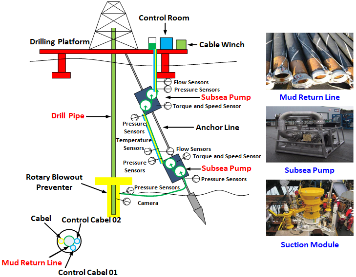
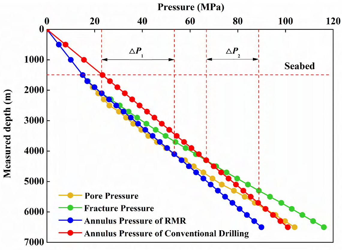
In 2003, BP America implemented commercial applications of the RMR system in the Caspian Sea. It is currently the most widely used and most successful DGD technology in the world. Compared with conventional offshore drilling, the RMR system has the following advantages: 1) The RMR system abandons the riser used in conventional offshore drilling, reducing drilling costs and requirements for drilling platforms and enabling the smaller drilling platforms to have the potential to drill in deep water. 2) As shown in Figure 2, compared to conventional offshore drilling, the RMR system enables the annulus pressure to be more within the safe pressure window, thus enabling the number of casings to be reduced. 3) The RMR system reduces the volume of mud used in the drilling process and reduces drilling costs. 4) The RMR system enables the cuttings at the bottom of the well to be lifted along the drilling fluid to the platform through the mud return line instead of being directly discharged to the seabed, thus meeting environmental requirements. 5) Because the RMR system uses a small diameter mud return line instead of a large diameter riser, the drilling fluid has a faster return flow rate. The RMR system has higher cuttings lifting efficiency than conventional offshore drilling.
The RMR system is still not widely used in the deepwater field, the main reasons are: 1) The technical principle of the subsea pump is complex, and it is not currently possible to manufacture a subsea pump suitable for using in deepwater field. 2) There are some difficulties in detecting and handling the kick, and the well control operation is complicated. 3) Because the drill pipe is directly exposed to seawater, the drill pipe needs to have higher corrosion resistance and fatigue strength.
Well control has always been a significant concern of offshore drilling engineering. Based on the drilling data of a vertical well in the South China Sea, this paper analyzes the factors affecting the annulus pressure of the RMR system by combining the dual-gradient pressure principle of the RMR
system. The main influencing factors include seawater depth, ESD of drilling fluid, cuttings concentration, and discharge capacity.
As the seasons and working waters change, the operating water depth will change accordingly. According to the dual- gradient pressure principle of the RMR system, the subsea pump adjusts the pump speed so that the pressure acting on the wellhead is equal to the subsea static pressure at that depth. Therefore, when the operating water depth changes, the pressure exerted by the subsea pump on the wellhead will also change accordingly, thereby affecting the annulus pressure. This condition is the most significant difference compared to conventional offshore drilling when analyzing the annulus pressure of the RMR system.
The volume of the drilling fluid in the annulus will change with the change of temperature difference and pressure difference. The change of drilling fluid volume will change the ESD of drilling fluid. The change of ESD of drilling fluid will change the ECD in the annulus. A change in the ECD can cause a change in the circulating liquid column pressure of the drilling fluid. Therefore, the effect of ESD of drilling fluid on annulus pressure is caused by temperature and pressure difference.
From the results of literature research, the influence of cuttings concentration on annular pressure is often neglected, but the reasons for the neglect are not explained. The cuttings concentration is a function related to the rate of penetration. In this paper, the influence of different cuttings concentrations on the annulus pressure is obtained through calculation. The calculation results show whether the cuttings concentration can be neglected in the calculation of the annulus pressure.
The flow rate of drilling fluid in the annulus varies with the discharge capacity change, resulting in different annulus pressure losses of drilling fluid in the annulus. Annulus pressure loss is an indispensable part of annulus pressure analysis. Based on the characteristics of the RMR system, the influence of different discharge capacities on annular pressure is analyzed in this paper.
Pressure field
The annulus pressure of the RMR system consists of three kinds of pressure: 1) The pressure exerted by the subsea pump on the wellhead, and it is also the inlet pressure of the subsea pump. 2) The circulating liquid column pressure is generated when the drilling fluid circulates in the annulus. 3) The pressure loss is caused by drilling fluid circulating in the annulus. The annulus pressure of the RMR system can be calcualted as shown in Equaton 1:
$$ P _ {\mathrm {a n n}} = P _ {\mathrm {i n l e t}} + P _ {\mathrm {m}} + \Delta P _ {\mathrm {f}} (1) $$ where _P_ann is the annulus pressure, MPa; _P_inlet is the inlet pressure of the subesea pump, MPa;_P_m is the circulating liquid column pressure; Δ_P_f is the annulus pressure loss, MPa.
The inlet pressure of the subesea pump can be written as shown in Equation 2:
inlet w w =0.00981 P h ρ where is the density of seawater, g/cm3; is the seawater depth, m.
The circulating liquid column pressure can be written as shown in Equation 3:
$$ P _ {\mathrm {m}} = 0. 0 0 9 8 1 \left[ \rho_ {\mathrm {m}} \left(1 - C _ {\mathrm {a}}\right) + \rho_ {\mathrm {c}} C _ {\mathrm {a}} \right] h _ {\mathrm {f}} \tag {3} $$ where ρm is the density of drilling fluid, g/cm3; ρc is the density of cuttings, g/cm3; _C_a is the cuttings concentration, dimensionless; _h_f is the formation depth, m.
When the fluid flow in the annulus is laminar, the annulus pressure loss can be written as shown in Equation 4:
( ) ( ) $$ \Delta P _ {\mathrm {f}} = \frac {4 h _ {\mathrm {f}} K}{\left(d _ {\mathrm {h}} - d _ {\mathrm {p o}}\right)} \left[ \frac {4 \left(2 n + 1\right) v _ {\mathrm {m , a n n}}}{n \left(d _ {\mathrm {h}} - d _ {\mathrm {p o}}\right)} \right] $$ $$ \Delta P _ {\mathrm {f}} = \frac {4 h _ {\mathrm {f}} K}{\left(d _ {\mathrm {h}} - d _ {\mathrm {p o}}\right)} \left[ \frac {4 (2 n + 1) v _ {\mathrm {m}}}{n \left(d _ {\mathrm {h}} - d _ {\mathrm {p o}}\right)} \right] $$ m,ann f f h po h po ( ) (4) When the fluid flow in the annulus is turbulent, the annulus pressure loss can be written as in Equation 5:
2 m f m,ann f h po $$ \Delta P _ {\mathrm {f}} = \frac {2 f \rho_ {\mathrm {m}} h _ {\mathrm {f}} v _ {\mathrm {m}} ^ {2}}{\left(d _ {\mathrm {h}} - d _ {\mathrm {p o}}\right)} $$ $$ \Delta P _ {\mathrm {f}} = \frac {2 f \rho_ {\mathrm {m}} h _ {\mathrm {f}}}{\left(d _ {\mathrm {h}} - a\right)} $$ (5) ( ) where K is the consistency coefficient of drilling fluid, Pa·sn; n is the fluidity index of drilling fluid, dimensionless; v_m,ann is the flow rate of drilling fluid in the annulus, m/s; _d_h is the diameter of wellbore, cm; _d_po is the outer diameter of drill pipe, cm; _f is the friction coefficient, dimensionless.
ECD can be written for annulus as shown in Equation 6:
$$ \mathrm {E C D} = \frac {\rho_ {\mathrm {w}} h _ {\mathrm {w}}}{h _ {\mathrm {f}}} + \left[ \rho_ {\mathrm {m}} \left(1 - C _ {\mathrm {a}}\right) + \rho_ {\mathrm {c}} C _ {\mathrm {a}} \right] + \frac {\Delta P _ {\mathrm {f}}}{h _ {\mathrm {f}}} $$ (6) ESD can be expressed with the Equation 7:
( ) m a c a $$ \mathrm {E S D} = \frac {\left[ \rho_ {\mathrm {m}} \left(1 - C _ {\mathrm {a}}\right) + \rho_ {\mathrm {c}} \right]}{1 + C _ {\mathrm {T}} \Delta T - C _ {P} \Delta} $$ C C $$ = \frac {\left[ \rho_ {\mathrm {m}} \left(1 - C _ {\mathrm {a}}\right) + \rho_ {\mathrm {c}} C _ {\mathrm {a}} \right]}{1 + C _ {\mathrm {T}} \Delta T - C _ {P} \Delta P} $$ (7) C T C P T $$ C _ {\mathrm {T}} = \frac {5 . 4 9 0 7 \times 1 0 ^ {- 4} \left[ \rho_ {\mathrm {m}} \left(1 - C _ {\mathrm {a}}\right) + \rho_ {\mathrm {c}} C _ {\mathrm {a}} \right]}{1 + 4 . 8 3 5 1 \times 1 0 ^ {- 3} \Delta T} $$ $$ 0 ^ {- 4} \left[ \rho_ {\mathrm {m}} \left(1 - C _ {\mathrm {a}}\right) + \rho_ {\mathrm {c}} C \right. $$ C C C T $$ \frac {7 \times 1 0 ^ {- 4} \left[ \rho_ {\mathrm {m}} \left(1 - C _ {\mathrm {a}}\right) + \rho_ {\mathrm {c}} C _ {\mathrm {a}} \right]}{1 + 4 . 8 3 5 1 \times 1 0 ^ {- 3} \Delta T} $$ (8) $$ C _ {\mathrm {P}} = 0. 5 6 3 6 \times 1 0 ^ {- 3} \left[ \rho_ {\mathrm {m}} \left(1 - C _ {\mathrm {a}}\right) + \rho_ {\mathrm {c}} C _ {\mathrm {a}} \right] \Delta P ^ {- 0. 1 3 9 4} \tag {9} $$ where C_T is the thermal expansion coefficient, dimensionless; _C_P is the elastic compression coefficient, dimensionless; Δ_T is the temperature difference between the drilling fluid at a certain depth and the platform, oC; ΔP is the pressure difference between the drilling fluid at a certain depth and the platform, MPa.
Cuttings concentration can be calculated via Equation 10:
$$ C _ {\mathrm {a}} = \frac {R O P}{3 6 0 0 \left(v _ {\mathrm {m , a n n}} - v _ {\mathrm {s}}\right) \left(1 - d _ {\mathrm {p o}} ^ {2} / d _ {\mathrm {h}} ^ {2}\right)} \tag {10} $$ $$ v _ {\mathrm {m}, \mathrm {a n n}} = \frac {4 0 Q}{\pi \left(d _ {\mathrm {h}} ^ {2} - d _ {\mathrm {p o}} ^ {2}\right)} \tag {11} $$ ( ) m,ann 2 2 h po $$ v _ {\mathrm {s}} = \mathrm {A} \sqrt {\frac {d _ {\mathrm {s}} \left(\rho_ {\mathrm {s}} - \rho_ {\mathrm {m}}\right)}{\rho_ {\mathrm {m}}}} $$ (12) where ROP is the rate of penetration, m/h; v_s is the setting velocity of cuttings in annulus, m/s; _Q is the discharge capacity, L/s; A is conversion coefficient, dimensionless; _d_s is the cutting diameter, cm.
Temperature Field
Assumptions
A drilling fluid control volume of length d_x_ is taken in the annulus, and the flow direction of drilling fluid is set to positive direction, and the following assumed conditions are made: 1) The temperature in any section of annulus perpendicular to the flow direction is uniform. 2) Ignore the heat conduction along the flow direction. 3) All physical properties are constants. 4) No heating measures were taken in the wellbore. Mathematical Model The physical model of heat transfer process of annulus is shown in Figure 3.
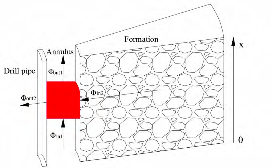
The heat injected from the lower surface of the control volume can be calculated via Equation 13:
in1 m p x q C t Φ = (13) The heat transfer from the formation to the drilling fluid in the annulus can be calculated via Equation 14:
$$ \Phi_ {\mathrm {i n 2}} = U _ {\mathrm {f a}} \pi \left(d _ {\mathrm {h}} - d _ {\mathrm {p o}}\right) \left(t _ {\mathrm {f o r}} - t _ {\mathrm {x}}\right) \mathrm {d x} \tag {14} $$ The temperature of the formation at depth x can be calculated via Equation 15:
$$ t _ {\mathrm {f o r}} = t _ {\mathrm {s}} + m (L - x) \tag {15} $$
The heat that flows from the upper surface of the control
volume can be calculated via Equation 16: $$ \Phi_ {\mathrm {o u t 1}} = q _ {\mathrm {m}} C _ {\mathrm {p}} t _ {\mathrm {x} + \mathrm {d x}} \tag {16} $$ The heat transfer from the drilling fluid in annulus to the drilling fluid in drill pipe can be calculated via Equation 17:
$$ \Phi_ {\mathrm {o u t 2}} = U _ {\mathrm {a p}} \pi \left(d _ {\mathrm {h}} - d _ {\mathrm {p o}}\right) \left(t _ {\mathrm {x}} - t _ {\mathrm {e}}\right) \mathrm {d x} \tag {17} $$ Combined with the boundary condition _t_x=0=_t_i, the calculation equation of the temperature of drilling fluid in annulus can be obtained as shown in Equation 18:
$$ t = A x + B e ^ {\mathrm {c x}} + D \tag {18} $$
$$ A = - \frac {m U _ {\mathrm {f a}}}{U _ {\mathrm {f a}} + U _ {\mathrm {a p}}} \tag {19} $$ fa fa ap U t U t mU q C B U U d d U U π $$ 3 = - \frac {U _ {\mathrm {f a}} t _ {\mathrm {i}} + U _ {\mathrm {a p}} t _ {\mathrm {e}}}{U _ {\mathrm {f a}} + U _ {\mathrm {a p}}} - \frac {m U _ {\mathrm {f a}} q _ {\mathrm {m}} C _ {\mathrm {p}}}{\pi \left(d _ {\mathrm {h}} - d _ {\mathrm {p o}}\right) \left(U _ {\mathrm {f a}} + U _ {\mathrm {a p}}\right) ^ {2}} \tag {20} $$ fa i ap e fa m p 2 fa ap h po fa ap ( )( ) ( ) ( ) fa ap h po m p U U C d d q C $$ C = - \frac {\left(U _ {\mathrm {f a}} + U _ {\mathrm {a p}}\right) \pi}{a C} \left(d _ {\mathrm {h}} - d _ {\mathrm {p o}}\right) \tag {21} $$ D=B (22) where U_fa is the heat transfer coefficient between the formation and the drilling fluid in annulus, W/(m2·oC); _U_ap is the heat transfer coefficient between the drilling fluid in annulus and the drilling fluid in drill pipe, W/(m2·oC); _t_i is the temperature of the drilling fluid at the bottom of well, oC; _t_e is the temperature of the drilling fluid in drill pipe, oC; _t_s is the surface temperature of formation, oC; _m is geothermal gradient, oC/100m; _q_m is the mass flow of drilling fluid through control volume, kg/s.
CFD Analysis
The temperature changes of the drilling fluid in the annulus at formation depth 500 m-1,000 m, 2,500 m-3,000 m, and 4,500 m-5,000 m were simulated. The basic parameters are shown in Table 1. The results of the CFD analysis are shown in Figure 4.
| Parameter | Data | Parameter | Data |
|---|---|---|---|
| Minimum annular velocity, m/s | 3.7 | Annulus width, m | 0.12 |
| Geothermal gradient, oC /100m | 4.2 | Formation density, kg/m3 | 3.1 |
| Heat transfer coefficient U , W/(m2• oC) fa | 430.3 | Heat transfer coefficient U , W/(m2• oC) ap | 152.7 |
Table 1: The results of the CFD analysis are shown in Figure 4.
(a) 4,500 m~5,000 m (b) 2,500 m~3,000 m (c) 500 m~1,000 m Figure 4: CFD analysis results of annulus temperature.
The temperature of the drilling fluid at the bottom of well is 67 oC. According to the result of CFD analysis, the temperature of drilling fluid at 4,500 m is about 80 oC, 90 oC at 3,000 m, 85 oC at 2,500 m, 70 oC at 1,000 m and 50 oC at 500 m. From the results of the CFD analysis, the temperature of drilling fluid in the annulus first increased and then decreased.
Calculation Results
The temperature distribution of drilling fluid in the annulus is calculated by using the established mathematical model. The calculation results are shown in Figure 5.
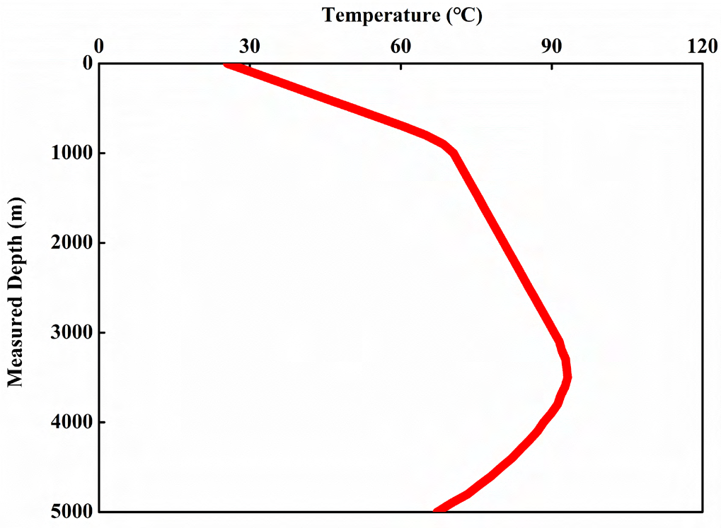
The calculation results are consistent with CFD analysis results, which show that the mathematical model established in this paper has sure accuracy.
From the calculation results, there is a tendency for the temperature of the drilling fluid in the annulus to rise first and then decrease. This is because when the drilling fluid begins to return in the annulus, Φ_in2 >Φout2, the temperature of the drilling fluid will rise. As the drilling fluid continues to flow in the annulus, Φin2 <Φ_out2, the temperature of the drilling fluid will drop.
Case study
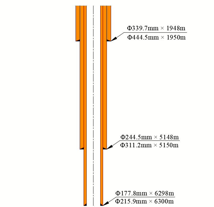
This paper’s calculations and analyses are based on drilling data from a vertical well in the South China Sea. Based on the drilling data of this well, the effects of seawater depth, ESD of drilling fluid, cuttings concentration, and discharge capacity on ECD and annulus pressure are analyzed in this section. The critical parameters of the well are shown in Table 2. The casing program of the well is shown in Figure 6. The calculation of this section is based on the size of the intermediate casing.
| Parameter | Data | Parameter | Data |
|---|---|---|---|
| Well depth, m | 6300 | Seawater depth, m | 1500 |
| Diameter of surface casing, m | 0.34 | Diameter of intermediate casing, m | 0.24 |
| Diameter of production casing, m | 0.18 | Diameter of drill pipe, m | 0.13 |
| Density of drilling fluid, kg/m3 | 1500 | Density of seawater, kg/m3 | 1020 |
| Density of cuttings, kg/m3 | 2500 | Surface temperature of seawater, ℃ | 20 |
| Geothermal gradient, ℃/100m | 4.2 | Circulation time, h | 8 |
| Rate of penetration, m/h | 7 | Discharge capacity, L/s | 45 |
Table 2: The casing program of the well is shown in Figure 6. The calculation of this section is based on the size of the interme
Effect of Seawater Depth
According to the dual-gradient pressure principle of the RMR system, the pressure exerted by the subsea pump on the wellhead is equal to the static pressure of the seawater at that depth. Therefore, the change in seawater depth mainly affects the pressure exerted by the subsea pump on the wellhead. By combining Equation 1 and Equation 6, the variation trend of ECD and annular pressure at seawater depths of 1,500 m, 2,000 m, 2,500 m, and 3,000 m is analyzed. The calculation results are shown in Figures 7 & 8.
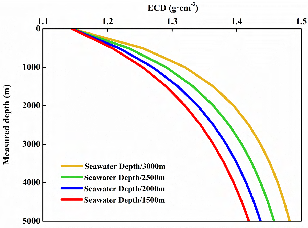
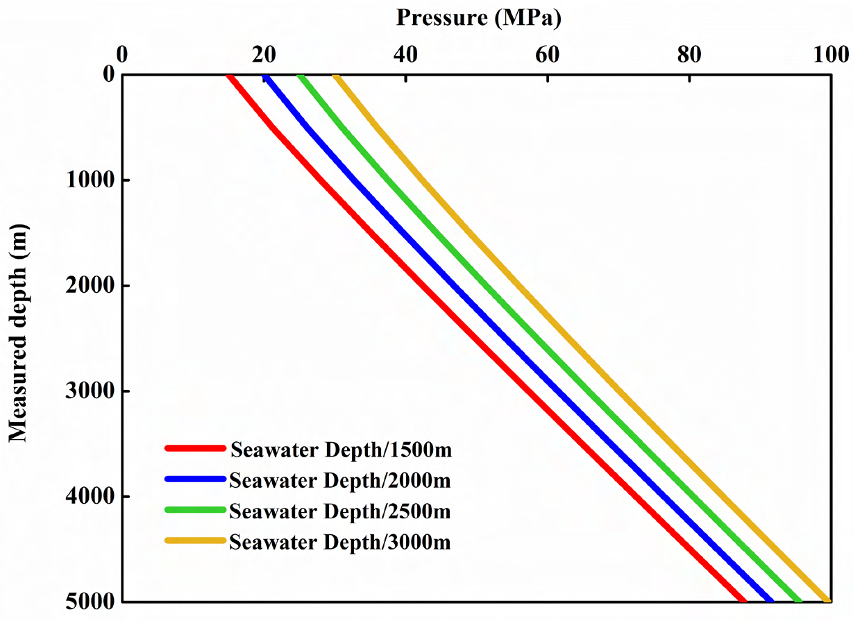
As can be seen from Figure 7 and Figure 8, as the seawater depth of the operating environment of the RMR system increases, the value of the ECD increase and the value of the annulus pressure increases.
This is because, as the seawater depth increases, the pressure _P_inlet acting on the wellhead increases, but the circulating liquid column pressure _P_m and annulus pressure loss Δ_P_f did not change. As a result, the ECD and annulus pressure increase.
From the above analysis, the inlet pressure of the subsea pump _P_inlet has an important influence on the change of the annulus pressure. Under the condition that the _P_inlet is constant, certain measures should be taken to regulate the ECD so that the annulus pressure can pass through the safe pressure window to a greater extent.
Effect of Cuttings Concentration
By combining Equation 3 and Equation 6, the effects of different cuttings concentration on ECD and annulus pressure are explored. The cuttings content was set to 5%, 7%, 9% and 11% respectively. The calculation results are shown in Figures 9 & 10.
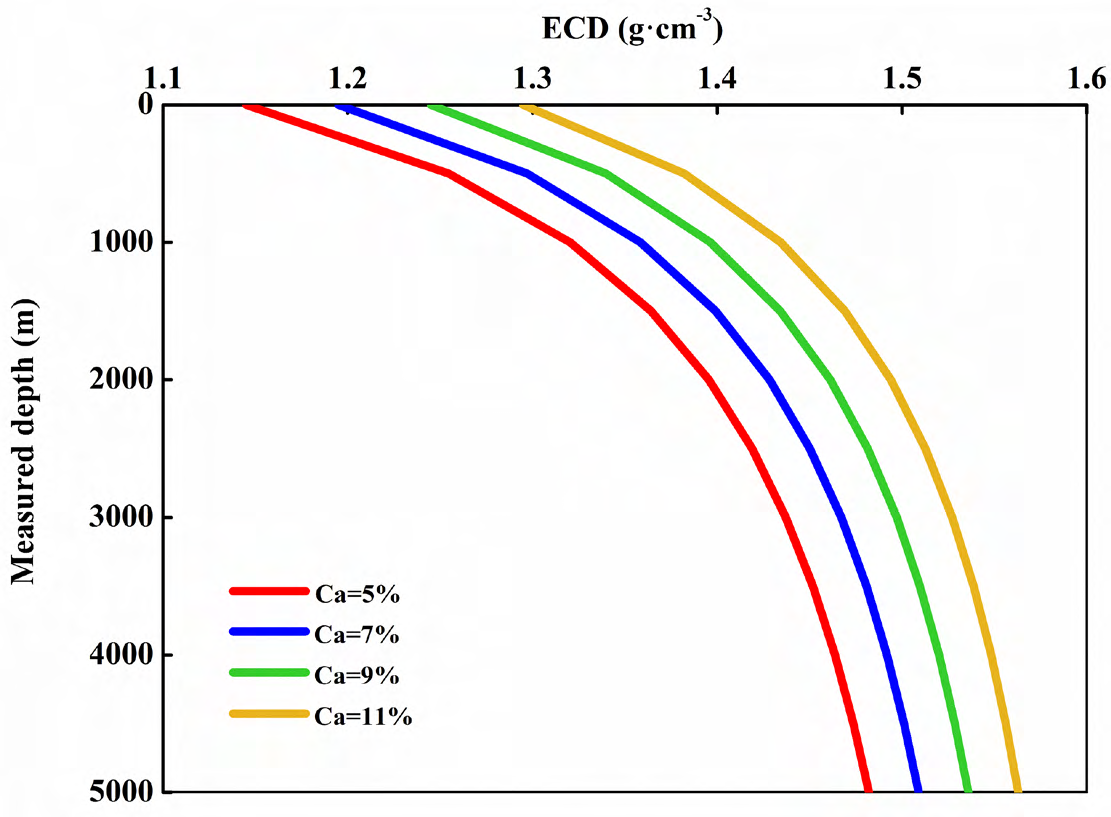
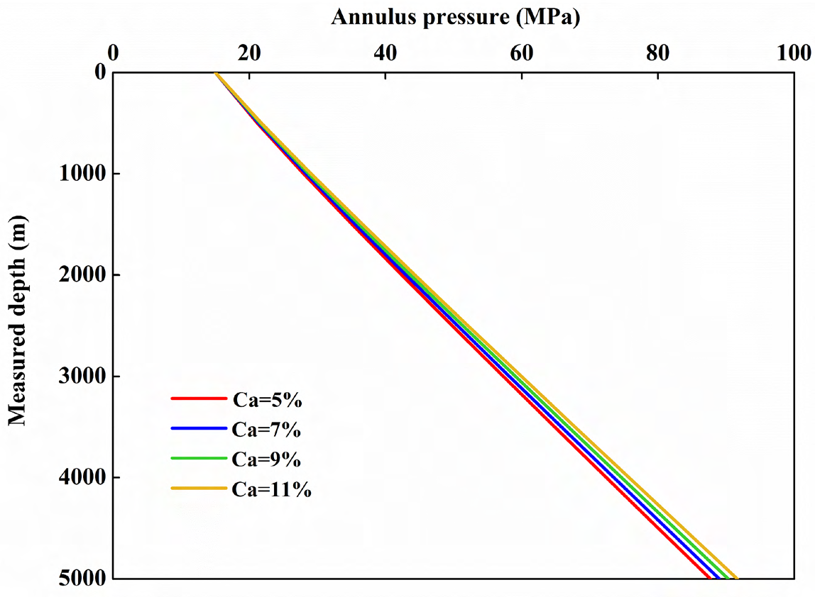
As can be seen from Figure 9 and Figure 10, as the cuttings concentration increases, the ECD and annulus pressure also increases. This is because, as the cuttings concentration increases, the circulating liquid column pressure _P_m increases, but inlet pressure of subsea pump _P_inlet and annulus pressure loss Δ_P_f did not change. As a result, the ECD and annulus pressure increase.
Effect of Discharge Capacity
By combining Equation 4 and Equation 5, it can be known that the discharge capacity mainly affects the annulus pressure loss. The discharge capacity is 45 L/s, 55 L/s, 65 L/s, and 75 L/s, respectively. The effects of different discharge capacities on ECD and annulus pressure are explored. The calculation results are shown in Figures 11 & 12.
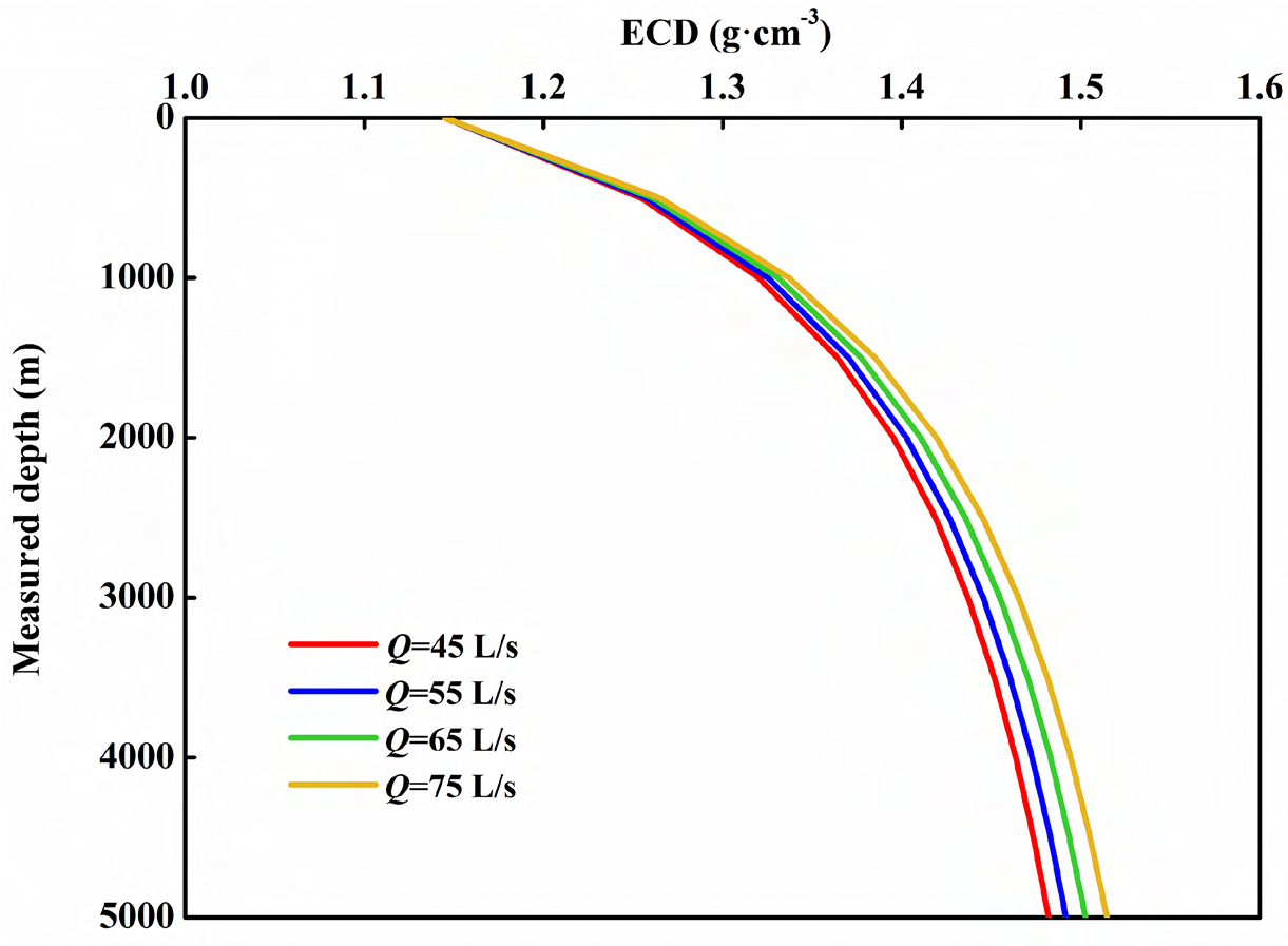
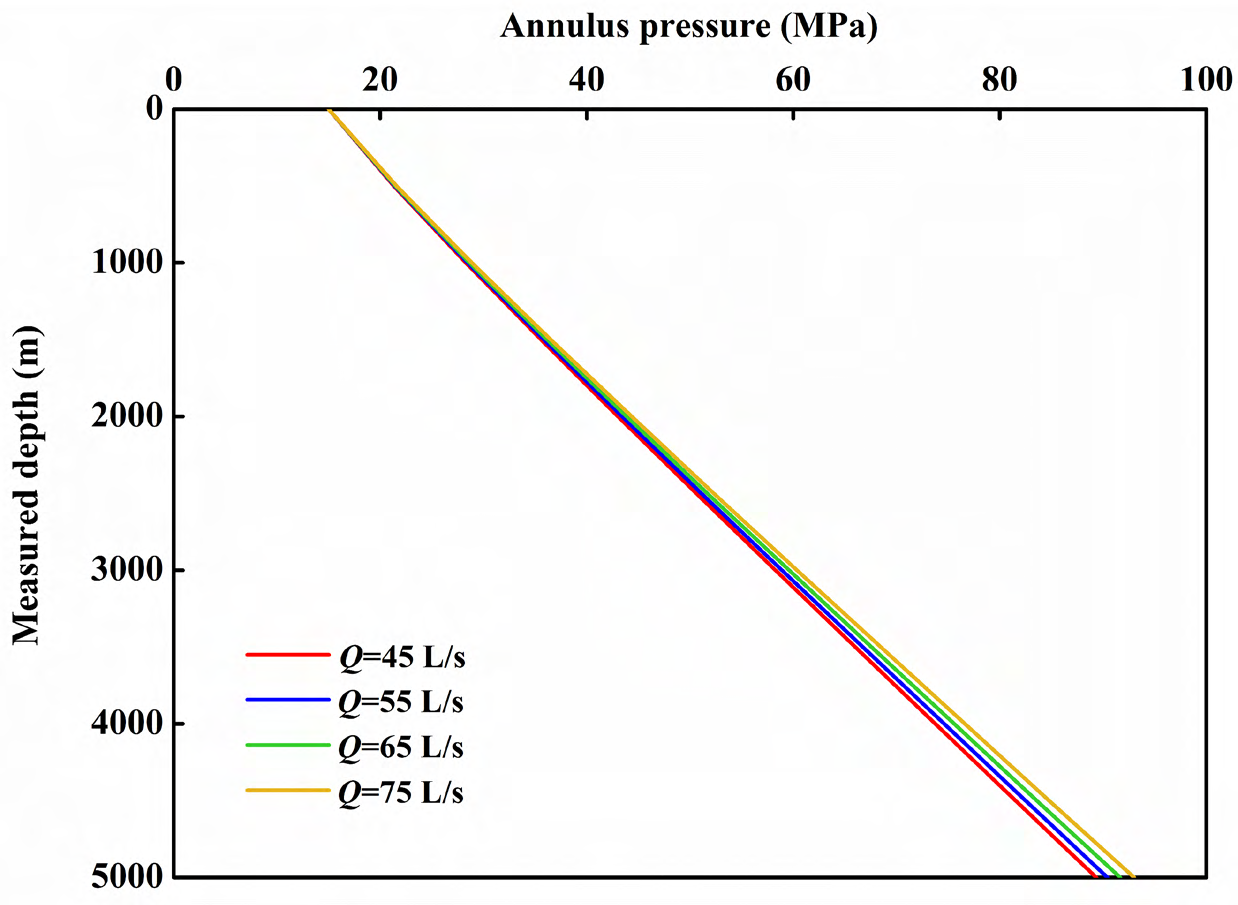
It can be seen from Figure 11 and Figure 12 that as the discharge capacity increases, the ECD will increase, and the annulus pressure will increase slightly.
The main reason is that as the discharge capacity increases, the flow velocity of the drilling fluid in the annulus becomes larger, and the pressure loss becomes larger. Combined with Equation 1 and Equation 6, it is obtained that the annulus pressure and the ECD is increased.
Conclusion
- The temperature of the drilling fluid in the annulus is calculated using a mathematical model of the thermal field within the annulus. Through the calculation results, the temperature of the drilling fluid in the annulus of the RMR system increases first and then decreases.
- As the seawater depth increases, the pressure _P_inlet acting on the wellhead increases, but the circulating liquid column pressure _P_m and annulus pressure loss Δ_P_f did not change. As a result, the ECD and annulus pressure increase.
- As the cuttings concentration increases, the circulating liquid column pressure _P_m increases, but inlet pressure of subsea pump _P_inlet and annulus pressure loss Δ_P_f did not change. As a result, the ECD and annulus pressure increase.
- As the discharge capacity increases, the flow velocity of the drilling fluid in the annulus becomes more extensive, and the pressure loss becomes larger, so the annulus pressure and ECD increase.
Acknowledgments
The authors thank the financial supports from the National Natural Science Foundation of China (No. 51274168), the National Key R&D Program of China (No. 2018YFC0310202), and the Southwest Petroleum University Graduate Research and Innovation Fund Key Program (No. 2020CXZD30).
Conflicts of Interest
The authors declare that they have no known competing financial interests or personal relationships that could have influenced the work reported in this paper.
References
-
Zhang J, Li X, Tang, X, Luo W (2019) Establishment and Analysis of Temperature Field of Riserless Mud Recovery System. Oil Gas Sci Technol 74(19): 1-9.
-
Li X, Zhang J, Tang X, Mao GZ, Wang PG (2020) Study on Wellbore Temperature of Riserless Mud Recovery System by CFD Approach and Numerical Calculation. Petroleum 6(2): 163-169.
-
Li X, Zhang J, Zhao HY, Zhang M, Sun XF, et al. (2020) Study on Lifting Efficiency of Cuttings in Return Line of Riserless Mud Recovery System. The 9th International Conference on Informatics, Environment, Energy and Applications, pp: 20-26.
-
Li X, Zhang J, Li CN, Li B, Zhao HY, et al. (2021) Variation characteristics of coal-rock mechanical properties under varying temperature conditions for Shanxi Linfen coalbed methane well in China. Journal of Petroleum Exploration and Production Technology 11(7): 2905- 2915.
-
Li X, Zhang J, Wu CJ, Hong TY, Zheng YD, et al. (2021) Experimental Research on the Effect of Ultrasonic Waves on the Adsorption, Desorption, and Seepage Characteristics of Shale Gas. ACS Omega 6(26): 17002- 17018.
-
Li X, Zhang J, Li RX, Qi Q, Zheng YD, et al. (2021) Numerical Simulation Research on Improvement Effect of Ultrasonic Waves on Seepage Characteristics of Coalbed Methane Reservoir. Energies 14(15): 4605.
-
Li X, Zhang J, Zheng YD, Li CN, Li ZL, et al. (2021) Experimental Research and Numerical Analysis of the Attenuation Law of Ultrasound Propagating in Shale. J Phys Conf Ser 1980: 012005.
-
Li X, Zhang J, Li CN, Chen WL, He JB, et al. (2022) Characteristic Law of Borehole Deformation Induced by the Temperature Change in the Surrounding Rock of Deep Coalbed Methane Well. Journal of Energy Resources Technology 144(6): 063003.
-
Zhang J, Zhao ZP, Li X, Zheng YD, Li CN, et al. (2021) Research on the mechanism of the influence of flooding on the killing of empty wells. Journal of Petroleum Exploration and Production Technology 11(9): 3751- 3598.
-
Godhavn J (2010) Control requirements for automatic managed pressure drilling system. SPE Drill Complet 25(3): 336-345.
-
Marcellinus A, Ojinnaka S, Joseph J (2018) Beaman Full- course drilling model for well monitoring and stochastic estimation of kick. Journal of Petroleum Science and Engineering 166: 33-43.
-
Rezk R (2013) Safe and Clean Marine Drilling with Implementation of “Riserless Mud Recovery Technology- RMR”. SPE Arctic and Extreme Environments Conference, Russia.
-
Stave R, Nordas P, Fossli B, French C (2014) Safe and Efficient Tophole Drilling using Riserless Mud Recovery and Managed Pressure Cementing. Offshore Technology Conference, Malaysia.
- Nigeria’s Vulnerability in the Face of Global Energy Policy
- A Simulation Study of Investigation of Optimum Oil Production Performance by Applying Various Gas Injection Methods in Oil Reservoir
- Characterization of Permo-Triassic Reservoirs through Thermal Maturity Assessment of Westphalian Source Rocks in the Cheshire Basin
- Influence of Microwax on the Rheological and Thermal Behaviour of a Wax Crude Oil
- Real-Time Monitoring and Performance Optimization of Steam Injection in Heavy Oil Reservoirs Using Fiber Optic Sensing and Integrated Predictive Simulation Models
- Rapid On-Site Determination of the Total Petroleum Hydrocarbon Content of Soils by Handheld Fourier Transform Near-Infrared Spectroscopy: Development of a Global, Site- and Scanner- Independent Calibration Model