An Innovative Method for Designing Smooth Catenary Well Trajectories in Extended-Reach Drilling

Chunkai Fu; Boyun Guo* and Xiao Cai

doi:10.23880/ppej-16000297

Petroleum & Petrochemical Engineering Journal Research Article 17 min read

An Innovative Method for Designing Smooth Catenary Well Trajectories in Extended-Reach Drilling

Chunkai Fu, Boyun Guo* and Xiao Cai^*

^* Corresponding author

ISSN: 2578-4846 10.23880/ppej-16000297 Received: February 25, 2022 Published: March 14, 2022

— views

13 references

4 figures

2 tables

PDF

Keywords

Analytical model Catenary trajectory Extended reach drilling Drag reduction

Abstract

A catenary well trajectory is known for its reduced drag and torque during drilling. Modern deflection tools have made it possible to drill catenary well trajectories efficiently, thanks to tool’s capacity of dynamic build rate that creates wellbore profile of varying curvature. However a method to design well trajectory with smooth transition from the kick-out point to the catenary section to reduce “dog-leg” and thus friction is still lacking. This paper presents a 2D mathematical solution to fill the gap. The solution uses equations of closed-form rather than numerical computations. The complete well trajectory profile involves a vertical section, a transitional arc section, a catenary section, and a horizontal/slant section. A case study is presented to compare the friction forces on the drill string in a catenary trajectory profile and a conventional trajectory profile of arc type. The calculation procedure of catenary trajectory design was realized in an MS Excel spreadsheet with direct inputs, which provides an excellent flexibility to meet well trajectory design requirement. The presented mathematical model is an easy-to-use and reliable tool for designing catenary well trajectories in extended-reach wells to minimize wellbore friction and thus increase well depth.

Chunkai Fu, Boyun Guo* and Xiao Cai

Introduction

Drilling technology has evolved rapidly in recent decades owing to the increasing need for extended reach or ultra- extended reach wells. Extended reach drilling (ERD) or ultra- extended reach drilling (u-ERD) is commonly deployed to boost the performance of reservoirs with limited production and help eliminate the need for extra drilling platforms [1]. An increasing number of ERD wells have been drilled since the 1990s when a wellbore needs to be drilled from an onshore well site to offshore reserves under the Poole Harbor [2]. In the late 1990s, the well M11 set a new world record with a reach of 10km, which was broken again in 2000 by Well M16 at 10,727 m depth and 11,278 m measured depth [2, 3]. The record depth of ERD is continuously broken with the rapid emergence of better tools, technologies, and well designs, which makes the drilling of u-ERD wells possible in the future.

As the measured depth increases during drilling, the difficulty of drilling increases due to the increased friction and torque imposed on the drill string by the wellbore. One effective approach to reducing excessive friction is to optimize well trajectory designs. The drill string acts like a rope with negligible bending rigidity due to the much greater length of drill string than its diameter. Therefore, if the wellbore can be drilled along to a catenary profile, the drill string should not touch the wellbore and thus there is no friction [4]. This is how the torque and drag of a catenary drill string are reduced in a catenary profile. However, unlike the traditional trajectory geometry of an arc, which has a constant build rate, the catenary well trajectory design requires a changing build rate as drilling proceeds. This technology was not available on a commercial scale by service companies such as Halliburton until recent years. Even with the right tool, the design of a catenary well trajectory, however, remains a challenge due to the lack of an efficient design methodology [1]. Therefore, the goal of this study is to propose a complete design methodology of an effective and efficient catenary well trajectory profile.

Despite the early introduction of catenary designs to the oil and gas industry back in 1985, the first attempts of this technology did not quite match its expected outcomes due to the absence of mature technology – dynamic build rate [5]. Several drilling trials were done using catenary profiles in China and most of the research efforts focused on the selection of wellbore profiles to reduce trip drag and friction [6]. The design methodology for the catenary trajectory in the majority of the current research in literature features a numerical solution, which in some cases requires a decent computational power to obtain reasonable results [7, 8, 9]. There have been several studies that focused on the design of catenary trajectories that featured 3D design for directional wellbores [10, 11]. Song et al. [12] provided a summary of the trajectory design methods, which includes the arc, the pendulum curve, the catenary curve, and the modified catenary curve. The challenge to design a complete catenary profile is how to transit from the vertical wellbore to the catenary section since the top of a catenary trajectory has a starting inclination greater than zero [4]. Some more recent studies provided a more efficient calculation method but a complete design of the trajectory profile is still lacking since only the catenary section is presented [13].

This paper presents a 2D model of catenary trajectory with smooth transitional section below the kick-out point and provides a complete wellbore trajectory design, which is simple and convenient to use. The solutions of the catenary design are in closed-forms and do not require extensive numerical estimations, which ensures that the trajectory is smooth in any condition without adjustment. A case study is also presented to compare the friction forces acting on the drill string by a catenary wellbore section and a conventional arc section.

Mathematical Model

This section summarizes the results of the characteristic parameters used for calculating the track coordinates of a catenary curve. Details can be found in the Appendix A. The complete workflow, which utilizes the results summarized here, is illustrated in the next section *Catenary Trajectory Design Workflow*.

In a two-dimension Cartesian coordinate system, a simple catenary curve can be expressed as the addition of two exponential functions:

$$y = a \cosh \left( \frac{x}{a} \right) = \frac{a}{2} \left[ e^{\frac{x}{a}} + e^{-\frac{x}{a}} \right]$$

where $a$ is the intercept of the catenary curve with the $y$ axis.

The relationship between horizontal displacement $S$ and depth $V$ can be represented as

$$V = V_{\text{end}} - \left\{ \frac{a}{2} \left[ e^{\frac{S - s_{\text{end}}}{a}} + e^{-\frac{S - s_{\text{end}}}{a}} \right] - a \right\}$$

The curvature of a function $V = f(S)$ can be expressed as

$$C = \frac{-1}{2a} \left[ e^{\frac{S - s_{\text{end}}}{a}} + e^{-\frac{S - s_{\text{end}}}{a}} \right] \left( 1 + \frac{1}{4} \left[ e^{\frac{S - s_{\text{end}}}{a}} - e^{-\frac{S - s_{\text{end}}}{a}} \right]^2 \right]^{\frac{1}{2}}$$

The build rate of the arc section or at the top of the catenary section in degrees per 100 feet is

$$B = 5,730C$$

The inclination angle can then be expressed as

$$\theta = \frac{\pi}{2} - \alpha = \frac{\pi}{2} - \arctan \left( \frac{dV}{dS} \right)$$

or

$$\theta = \frac{\pi}{2} - \arctan \left\{ -\frac{1}{2} \left[ e^{\frac{S - s_{\text{end}}}{a}} - e^{-\frac{S - s_{\text{end}}}{a}} \right] \right\}$$

Catenary Trajectory Design Workflow

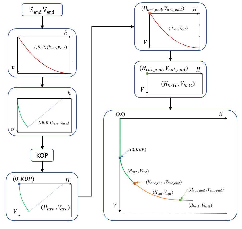
The design workflow of the complete trajectory of a horizontal wellbore is shown in Figure 1. The total length $(S_{\text{end}})$ and height $(V_{\text{end}})$ of the catenary section are used as inputs to calculate the inclination angle $(\theta)$, the build rate $(B)$, the radius of curvature (R), and the trajectory of the catenary curve( ) , cat cat h ν . The lower cases of h and ν indicate that the coordinates are local and relative to the beginning of the catenary section, whose coordinate is (0, 0). The inclination angle, build rate, and radius of curvature are constantly with depth. A catenary curve has a beginning inclination angle that needs to be connected smoothly to the arc section above it. To ensure a smooth connection, The curvature and inclination angle of the arc section needs to be configured the same as those that are at the beginning of the catenary section. With curvature and inclination angle, the coordinates of the arc section can be obtained ( ) , arc arc h ν from Equation (2). The horizontal displacement and the vertical depth are also relative to the beginning of the arc section. Since the total vertical depth of the wellbore is known, the kickoff point (KOP) can be obtained by subtracting the total heights of the arc and catenary sections from the total vertical depth.

After the KOP is determined, the coordinates relative to the open hole at the surface can be obtained. The upper cases of H and V indicate that the coordinates are global and relative to the position of the open hole, which is assumed to be (0, 0). The coordinate of the KOP is (0, KOP). The horizontal displacement of the arc section after the KOP can be expressed as $$ H _ {a r c} = R - R ^ {*} \cos (\theta) $$ (6) $$ V _ {a r c} = K O P + R ^ {*} \sin (\theta) \tag {7} $$ where R is the radius of curvature of the arc section; θ is the inclination angle of the arc section; KOP is the depth of the kickoff point.

After the global coordinates of the arc section are obtained, the global coordinates of the catenary section can be calculated as $$ V _ {c a t} = V _ {a r c _ {-} e n d} + v _ {c a t} \tag {8} $$ $$ H _ {c a t} = H _ {a r c _ {-} e n d} + h _ {c a t} \tag {9} $$ where _ arc end V is the global vertical depth of the arc section;

_ arc end H is the global horizontal displacement of the arc section.

After the coordinates of the catenary section are obtained, the position of the horizontal wellbore can be determined as $$ H _ {h r t l} = H _ {c a t \_ e n d} + L _ {h r t l} \tag {10} $$ $$ V _ {h r t l} = V _ {c a t _ {-} e n d} \tag {11} $$ where cat end H is the position of the end of the catenary section; cat end V is the depth of the end of the catenary section;

hrtl L is the length of the horizontal wellbore. Plotting the coordinates of each section, the wellbore trajectory can be obtained shown in the last step of the flow chart.

Figure 1: The total length $(S_{\text{end}})$ and height $(V_{\text{end}})$ of the catenary section are used as inputs to calculate the inclination angle $(\theta)$, the build rate $(B)$, the radius of curvature (_R_), and the trajectory of the catenary curve( ) , cat cat h ν . The lower cases of _h_ and ν indicate that the coordinates are local and relative to the beginning of the catenary section, whose coordinate is (0, 0). The inclination angle, build rate, and radius of curvature are constantly with depth. A catenary curve has a beginning inclination angle that needs to be connected smoothly to the arc section above it. To ensure a smooth connection, The curvature and inclination angle of the arc section needs to be configured the same as those that are at the beginning of the catenary section. With curvature and inclination angle, the coordinates of the arc section can be obtained ( ) , arc arc h ν from Equation (2). The horizontal displacement and the vertical depth are also relative to the beginning of the arc section. Since the total vertical depth of the wellbore is known, the kickoff point (KOP) can be obtained by subtracting the total heights of the arc and catenary sections from the total vertical depth. — Figure 1: The total length $(S_{\text{end}})$ and height $(V_{\text{end}})$ of the catenary section are used as inputs to calculate the inclination angle $(\theta)$, the build rate $(B)$, the radius of curvature (R), and the trajectory of the catenary curve( ) , cat cat h ν . The lower cases of h and ν indicate that the coordinates are local and relative to the beginning of the catenary section, whose coordinate is (0, 0). The inclination angle, build rate, and radius of curvature are constantly with depth. A catenary curve has a beginning inclination angle that needs to be connected smoothly to the arc section above it. To ensure a smooth connection, The curvature and inclination angle of the arc section needs to be configured the same as those that are at the beginning of the catenary section. With curvature and inclination angle, the coordinates of the arc section can be obtained ( ) , arc arc h ν from Equation (2). The horizontal displacement and the vertical depth are also relative to the beginning of the arc section. Since the total vertical depth of the wellbore is known, the kickoff point (KOP) can be obtained by subtracting the total heights of the arc and catenary sections from the total vertical depth.

Case Study

Catenary Profile

It is known that the shape of the wellbore profile is determined by a set of characteristic parameters i.e., build rate, inclination angle, the radius of curvature, section length, and height and there are numerous combinations of these parameters. It is therefore necessary to compare the alleged best design with other profiles when drag and friction during trips are used as the decision criteria.

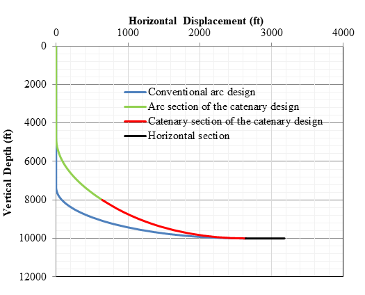
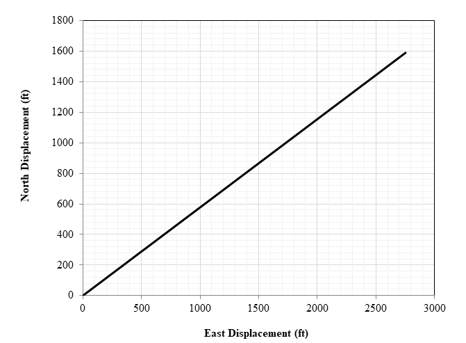
In this section, the catenary trajectory profile is calculated and illustrated together with a conventional profile that features an arc design. It is assumed that the two design profiles have the same surface well location and horizontal wellbore entry point. The geometrical data for the catenary design and the arc design are shown in Table 1 and Table 2. The illustrations of the two profiles are shown in Figure 2, and the plan view of the catenary design is shown in Figure 3. The horizontal section is intentionally made short, which could be much longer in reality. Notice that the horizontal and vertical axes are not at the same scale.

Description	Value	Unit
Total measured depth	30,000	ft
Target depth	10,000	ft
Vertical displacement in the catenary section ($V_{end}$)	2,000	ft
Horizontal displacement in the catenary section ($S_{end}$)	2,000	ft
Azimuth	60	degrees
Parameter a	1238	ft
Inclination angle at top of catenary section	22.43	deg
Radius of curvature at top of catenary section	8,470	ft
Build rate at the top of catenary section	0.6765	deg/100 ft
Vertical displacement in the arc section	3,231	ft
Kick off point (KOP)	4,769	ft
Arc length of the arc section	3,315	ft

Table 1: Geometrical Data for the Catenary Design.

Description	Value	Unit
Target depth	10,000	ft
Azimuth	60	degrees
Radius of curvature	3,179	ft
Vertical displacement in the arc section	3,179	ft
Kick-off point	7,359	ft

Table 2: Geometrical Parameters for the Arc Design.

The radius of curvature on the arc section is determined by the horizontal distance between the well location and the entry point of the horizontal section, which is 3179 ft. The KOP for the arc design is calculated by subtracting vertical depth by the radius of curvature.

Click to enlarge

Figure 2: Side views of the catenary and arc trajectory designs.

Click to enlarge

Figure 3: The horizontal section is intentionally made short, which could be much longer in reality. Notice that the horizontal and vertical axes are not at the same scale.

Friction Analysis

It is assumed that there is no friction in the catenary section on the drill string and the major difference in friction on the drill string between these two profiles is on the curve section, so only the frictions on the arc sections are compared. The friction on the arc section of a drill string can be expressed as $$ f _ {\theta} = \mu N _ {\theta} \tag {12} $$ where Nθ is the normal force on the drill string, µ is the friction coefficient, and fθ is frictional force expressed by $$ f _ {\theta} = \mu W _ {\theta} \sin (\theta) \tag {13} $$ where Wθ is the weight of the drill string element in the arc section, θ is the inclination angle of the element.

The total friction over an arc section can be expressed as $$ F _ {\theta} = \int_ {\theta_ {1}} ^ {\theta_ {2}} \mu w _ {c} \sin (\theta) R d \theta \tag {14} $$ ( )

1 sin c F w Rd θ

2 where c w is the unit weight of the drill string, R is the radius of curvature of the arc section, 1 θ and 2 θ are the inclination angles at the ends of the arc section. Integration of Equation (14) gives, ( )

1 cos c F Rw θ $$ F _ {\theta} = \mu R w _ {c} \left[ - \cos (\theta) \right] _ {\theta_ {1}} ^ {\theta_ {2}} \tag {15} $$

2 or ( ) ( ) 1 2 cos cos c F Rw θ µ θ θ   = −   (16)

The catenary design still utilizes an arc section for a smooth transition into the catenary section, but with a much shorter measured depth.

For the catenary design,

$$ \theta_ {1} = 0, \mathrm {a n d} \theta_ {2} = 2 2. 4 3 ^ {0}. $$

. The friction

on the arc section of the catenary design is $$ F _ {\theta} = 8 4 7 0 \mu w _ {c} \left[ \cos (0) - \cos \left(2 2. 4 3 ^ {0}\right) \right] = 6 4 1 \mu w _ {c} $$ For the arc design,

$$ n, \theta_ {1} = 0, \mathrm {a n d} \theta_ {2} = 9 0 ^ {0}. $$

. The friction on the

arc section of the arc design is $$ F _ {\theta} = 3 1 7 9 \mu w _ {c} \left[ \cos (0) - \cos \left(9 0 ^ {0}\right) \right] = 3 1 7 9 \mu w _ {c} $$ The ratio of friction force in the arc section of the conventional arc-design to that in the arc section of catenary design is (3179)/ (641) = 4.96. The friction in the angle- building section of the well trajectory is reduced by (3179- 641)/ (3179) = 0.7984, or 79.84%.

Conclusion

An analytical model is derived in this study for designing well trajectory profiles with a smooth transition from the pick-out point to the catenary section. The analytical model uses equations of closed-form, eliminating numerical computations for smoothness adjustment.
Result of case studies shows that the friction force acting on the drill string by a catenary section with a smooth transition is about 20% of that by an arc section in the angle-building section of an extended reach well. This will allow the extended-reach well to be drilled deeper.
The calculation procedure of the new catenary well trajectory design is carried out in an MS Excel spreadsheet with direct inputs and Macro.

The spreadsheet provides an efficient and flexible means of designing well trajectories for extended-reach drilling.

Nomenclature

a = Intercept of the catenary curve with the y axis.

Vend = Vertical height of the catenary section.

Send = Horizontal length of the catenary section.

C = Curvature of the curved section.

B = Build rate for the curved section.

I = Inclination angle (in Figure 1)

S = Horizontal coordinate, relative to the end of arc section.

V = Vertical coordinate, relative to the end of arc section.

KOP = Kickoff point or the depth of the kickoff point.

_ arc end V = Vertical depth of the arc section.

_ arc end H = Horizontal displacement of the arc section.

_ cat end H = Position of the end of the catenary section.

_ cat end V = Depth of the end of the catenary section.

hrtl L = Length of the horizontal wellbore.

Nθ = Normal force on the drill string.

µ = Friction coefficient.

Fθ = Total friction on the drill string.

fθ = Friction on the drill string.

Wθ = Weight of the drill string of the arc section.

α = Slope angle.

c w = Unit weight of the drill string.

θ = Inclination angle.

Acknowledgment

This research was partially supported by the U.S. Department of Energy project “Tuscaloosa Marine Shale Laboratory” (Project No. DE-FE0031575).

References

Liu X, Samuel R (2009) Catenary well profiles for ultra extended- reach wells. SPE Annual Technical Conference and Exhibition, New Orleans, Louisiana.
Robertson N, Hancock S, Mota L (2005) Effective Torque Management of Wytch Farm Extended Reach Sidetrack Wells. SPE Annual Technical Conference and Exhibition, Dallas, Texas, USA.
Meader T, Allen F, Riley G (2000) To the Limit and Beyond - The Secret of World-Class Extended Reach Drilling Performance at Wytch Farm. IADC/SPE Drilling Conference, New Orleans, Louisiana, USA.
Aadnoy BS, Fabiri VT, Djurhuus J (2006) Construction of Ultra-long Wells Using a Catenary Well Profile. IADC/ SPE Drilling Conference, Miami, Florida, USA.
McClendon RT, Anders EO (1985) Directional Drilling Using the Catenary Method. SPE/IADC Drilling Conference, New Orleans, Louisiana, USA.
Du CW, Zhang YJ (1987) The New Technology in Directional Drilling Catenary Profile. Oil Drilling & Production Technology 9(1): 17-22.
Han ZY (1987) The Method of Practical Design of Catenary-shape Profile. Oil Drilling & Production Technology 9(6): 11-17.
Payne ML, Cocking DA, Hatch AJ (1994) Critical Technologies for Success in Extended Reach Drilling. SPE Annual Technical Conference and Exhibition, New Orleans, Louisiana, USA.
Liu XS (2007) Study on the Methods for planning a Catenary Profile. Natural Gas Industry 27(7): 73-75.
Chen W, Ling J A (2004) New Computation Model for ERD Catenary Trajectory Design. Computer Engineering S1.
Joshi DR, Samuel R (2017) Automated geometric path correction in directional drilling. SPE Annual Technical Conference and Exhibition, San Antonio, Texas, USA.
Song Z, Gao D, Li R (2006) Summary and Optimization of Extended-Reach-Well Trajectory Design Method. Journal of Petroleum Drilling Technologies 34(5): 24-27.
Wiśniowski, R, Skrzypaszek, K, Lopata, P, Orlowicz G (2020) The Catenary Method as an Alternative to the Horizontal Directional Drilling Trajectory Design in 2D Space. Energies 13(5): 1112. Appendix A: Mathematical Formulation of Catenary Well Trajectory In a two-dimension Cartesian coordinate system, a simple catenary curve can be expressed as the addition of two exponential functions: $$ \gamma = a \cosh \left(\frac {x}{a}\right) = \frac {a}{2} \left[ e ^ {\left(\frac {x}{a}\right)} + e ^ {\left(\frac {- x}{a}\right)} \right] $$ x x a a x a y a e e a (A1) cosh 2 where a is the intercept of the catenary curve with the y axis. Figure 4 shows a catenary curve in two Cartesian coordinates. The x-y coordinates are used to illustrate the mathematical relationship between x and y while the S-V coordinates are used to illustrate the horizontal and vertical displacement of the drill bit during drilling. Let us assume a common scenario where the direction of the exit of the catenary section is horizontal. The starting point of the catenary section is represented by a red star and the end of it a blue star. It is easy to obtain that the tangent for point A is zero and it is where the horizontal wellbore is connected and extended. Drilling through the horizontal section after pint A is an easy task due to the same zero tangent of the catenary exit and horizontal entry. However, for the entry point of the catenary curve, there is a starting angle, which means that the vertical wellbore will not drill directly into the catenary and so a transition angle-making arc section will be needed. For now, let us focus on how to represent the horizontal and vertical displacement of drill bit along catenary ∂ OA . [INLINE_FIGURE:6:0] Figure 4: Geometry parameters of a catenary curve. Moving the horizontal axis up by _a_ and the vertical axis to the left by , the distance from a point on the catenary curve to the horizontal axis can be represented as $$ ' = \frac {a}{2} \left[ e ^ {\left(\frac {s - s _ {e n d}}{a}\right)} + e ^ {\left(\frac {s - s _ {e n d}}{a}\right)} \right] - a $$ end end s s s s a a a y e e a ' 2 (A2) The vertical depth from point O to the catenary curve can be therefore represented as $$ V = V _ {e n d} - y ^ {\prime} \tag {A3} $$ which is $$ = V _ {e n d} - \left\{\frac {a}{2} \left[ e ^ {\left(\frac {s - s _ {e n d}}{a}\right)} + e ^ {\left(\frac {s - s _ {e n d}}{a}\right)} \right] - a \right\} $$ end end s s s s end a V V e e a a a (A4) 2 where _a_ is numerically solved from boundary condition _V_ = 0 at _S_ = 0 using Equation (A5) $$ = \frac {a}{2} \left[ e ^ {\left(\frac {- s _ {e n d}}{a}\right)} + e ^ {\left(\frac {s _ {e n d}}{a}\right)} \right] - a $$ end end s s end a V e e a a a (A5) 2 The curvature of the arc section before the catenary section is fixed, but the curvature of the catenary section is changing as drilling continues. The curvature of a function _V = f(S)_ can be expressed as 2 d V dS C 2 $$ \cdot = \frac {d S ^ {2}}{\left(1 + \left(\frac {d V}{d S}\right) ^ {2}\right) ^ {\frac {3}{2}}} $$ (A6) 3 2 2 1 dV dS where     − −   −              = − −     end end s s s s 1 2 a a dV e e dS (A7) and $$\frac{d^2V}{dS^2} = -\frac{1}{2a} \left[ e^{\left( \frac{s-s_{md}}{a} \right)} + e^{\left( \frac{s-s_{md}}{a} \right)} \right]$$ The curvature can then be expressed as $$C = \frac{-\frac{1}{2a} \left[ e^{\left( \frac{s-s_{md}}{a} \right)} + e^{\left( \frac{s-s_{md}}{a} \right)} \right]}{1 + \left( -\frac{1}{2} \left[ e^{\left( \frac{s-s_{md}}{a} \right)} - e^{\left( \frac{s-s_{md}}{a} \right)} \right]^2 \right]^{\frac{3}{2}}}$$ The radius of curvature is $$R = \frac{1}{C}$$ The build rate of the arc section or at the top of the catenary section in degree per 100 feet is $$B = 5,730C$$ The inclination angle can then be expressed as $$I = \frac{\pi}{2} - \alpha = \frac{\pi}{2} - \arctan \left( \frac{dV}{dS} \right) = \frac{\pi}{2} - \arctan \left\{ -\frac{1}{2} \left[ e^{\left( \frac{s-s_{md}}{a} \right)} - e^{\left( \frac{s-s_{md}}{a} \right)} \right] \right\}$$

← Previous Article Mathematical Modeling of Heat Transfer from Geothermal Zones to Natural Gas Hydrate Reservoirs Next Article → Offset Wells Data Analysis and Thermal Simulations Improve the Performance of Drilling HPHT Well

An Innovative Method for Designing Smooth Catenary Well Trajectories in Extended-Reach Drilling

Chunkai Fu, Boyun Guo* and Xiao Cai

Introduction

**Mathematical Model**

**Catenary Trajectory Design Workflow**

Case Study

Catenary Profile

Friction Analysis

Conclusion

Nomenclature

Acknowledgment

References

Cite this article

Mathematical Model

Catenary Trajectory Design Workflow