Thermal Operational Map of an ESP-In-Skid Motor: A CFD Approach
The production of oil in offshore wells has used artificial lifting methods in order to maintain or increase production. In this sense, several established methods for onshore production, such as electrical submersible pumping (ESP), have been implemented in offshore scenarios and, as a consequence, new challenges and needing improvements to optimize production in this type of environment had to be faced. Many studies concern the gas-liquid flow inside de pump but avoid include the motor and its thermal management. In this context, this study focused to assess the complex flow around an ESP motor installed in subsea skids on the seabed (Skid-ESP) through the analysis of their operational and geometric conditions using a computational fluid dynamics (CFD) tool. The main question is: is it possible to create a thermal operational map of the motor in function of motor frequency with CFD tools? The Volume-of-Fluid (VOF) model was applied together with a homogeneous heat transfer (shared temperature field among phases) coupled to the heat conduction inside motor. This approach is known as Conjugate Heat Transfer (CHT). The ESP motor is modeled as a homogeneous and isotropic body with constant volumetric heat generation. The flow analysis was performed applying the model on an industrial scale with incompressible oil and gas in in-situ conditions and considering the heat transfer between the fluid mixture and the its boundary conditions (seawater constant temperature of 4°C and variable motor heat flux as function of motor frequency). The motor frequency range considered was between 40 and 60 Hz. Since the model used was 3D, hot spots were observed at the low part of near seal motor side for gas volume fraction above 3.5%. The employed methodology was able to determine the thermal operational map with a 5% average deviation from field data.
Introduction
Oil production systems in offshore wells often require methods to maintain or increase production such as artificial lift methods, such as ESP (electrical submersible pumping) or PCP (progressive cavity pumping). In conventional ESP systems, the electric motor-centrifugal pump assembly is located inside the production column [1]. In both onshore and offshore situations, ESP is economically disadvantageous due to high intervention operation cost, since it is necessary to stop production to remove the production column [2]. According to Urban, et al. [3], the first alternative system for using ESP pumps outside the well, and therefore decoupled from the production column, is known as MOBO (subsea pumping module), where the pump is installed at the bottom of a false well in the seabed. According to Roberto, et al. [4], a new system was subsequently developed, called the ESP-in-skid represented by Figure 1. In the ESP-in-skid the pumping device is housed in the seabed a few meters ahead a subsea wellhead downstream, whose main purpose is to reduce the subsea satellite well equipment intervention costs. The main components of the ESP-in-skid are: (1) the pump module (ESP in pink inside a skid, in yellow) and (2) the flowbase (or pump support) represented in Figure 1. According to Roberto, et al. [4], the flow base component design allows an installation and recovery independent of the pumping module. The flow base has a bypass module to maintain production during a pump module intervention. This system consists of vertical connectors (VCM - Vertical Connectors Module), hydraulic actuators for opening and closing valves in the event of failure, ROV panel, production lines, umbilical connectors (UTM - Umbilical Termination Module) and installation tool. The pumping module houses two ESP capsules in an “X” configuration, with 5 ° inclination in relation to the horizontal plane and they are connected in series [4].
![Figure 1: In the ESP-in-skid the pumping device is housed in the seabed a few meters ahead a subsea wellhead downstream, whose main purpose is to reduce the subsea satellite well equipment intervention costs. The main components of the ESP-in-skid are: (1) the pump module (ESP in pink inside a skid, in yellow) and (2) the flowbase (or pump support) represented in Figure 1. According to Roberto, et al. [4], the flow base component design allows an installation and recovery independent of the pumping module. The flow base has a bypass module to maintain production during a pump module intervention. This system consists of vertical connectors (VCM - Vertical Connectors Module), hydraulic actuators for opening and closing valves in the event of failure, ROV panel, production lines, umbilical connectors (UTM - Umbilical Termination Module) and installation tool. The pumping module houses two ESP capsules in an “X” configuration, with 5 ° inclination in relation to the horizontal plane and they are connected in series [4].](/fulltextimages/9039/fig_1.png)
According to the study by Tarcha, et al. [2], the main advantages offered by ESP-in-skid are: lower ESP installation costs and easier intervention operations, as the system is outside the well; the production loses are reduced due to the two pumps serial configuration with a bypass. When an intervention is necessary, one of the ESPs may continue to produce and the system operation can be maintained during ROV interventions. On the other hand, the main system disadvantage is the recommendation for pumping the production fluid with a maximum gas-fraction that is allowed to operate the ESP pump, which are 35% for the ESP-in-skid and 40% for the MOBO. The use of the ESP in subsea satellite wells with a high gas concentration causes pump problems and reduces their average time between failures (MTBF). Some identified problems are associated with the gas lock phenomenon, characterized by the passage of large gas-fractions in conventional pumps leading to non- ideal operating conditions [5]. A high gas-fraction may also overheat the ESP motor leading to a poor motor cooling, which also reduces the average time between failures (MTBF).
Most fluid flow ESP studies Ofuchi E, et al. [6] Deshmukh D, et al. [7] Peng L, et al. [8] are focused in the isothermal flow inside the centrifugal pump. Few studies are found in the literature with the aim to model the thermal ESP motor behavior.
Rodriguez, et al. [9] performed a parametric analysis using the commercial code CFX 4.2 to verify the equipment thermal behavior following the classic rule of shroud/motor configuration for heavy oils (viscosity of 78 cP @ 320 K). The authors concluded that for that oil a speed of 0.85 m/s (2.8 ft/s) should be maintained instead of 1 ft/s. In addition, the inclusion of slots in the shroud to redistribute the flow may improve the thermal motor cooling.
O’Bryan, et al. [10] validate and optimize the temperature field inside an electric motor using a CFD tool to model with a 5% experimental margin concordance. The simulation results were used to optimize the electric motor design.
Lin, et al. [11] developed a coupled flow and heat transfer model which was compiled in C code and validated by field measurements. The numerical calculation results show that marine environment factors, the heat emitted by pump and cable, and the Joule-Thomson effect have significant impact on the wellbore temperature and pressure distribution. When temperature decreases due to a low water cut condition and high gas-oil ratio, a resulted gas-fraction increase and a fluid density decrease will reduce the ESP pump pressure.
Betonico, et al. [12] studied the oil viscosity and water cut effect on the maximum motor temperature. The results showed the motor temperature rises as the motor speed is increased. It was also shown that neglecting the effect of the thermal boundary layer development on the motor surface may result in an overheated motor prediction where actually, the motor maximum temperature is much lower than its upper limit. It was observed that fully developed temperature profile models suffer from inaccuracy when used in viscous oil applications due to their great thermal entry length.
Martins, et al. [13] employed a Computational Fluid Dynamics (CFD) code to solve the governing equations of the turbulent heat transfer single-phase flow in the ESP motor annulus space. The standard kappa-epsilon model with the Enhanced Wall Treatment (FLUENT, 2013) is used as a turbulence closure problem. This study considered flow rates range of 2200-4200 m³/d (representing Reynolds numbers range of 27,000-133,000 approximately), Prandtl numbers 7-37, together with the wall boundary conditions of the constant temperature on the motor surface (130 °C) and capsule (quiescent seawater @ 4 °C). The authors observed that if the constant heat flux condition were used, the motor temperature would have lower values at the beginning and higher at the end of the geometry. Therefore, the higher the Nusselt number, the greater the heat transfer, which intensifies the electric motor cooling.
None of the previous works presented an analysis of the ESP motor thermal management at the seabed conditions since ESP are usually installed in the bottomhole. Therefore, this study aims to construct a thermal operational map of a ESP motor installed in the seabed through the analysis of real operational and geometric conditions using computational fluid dynamics (CFD) tools. The CFD model considers incompressible two-phase turbulent flow model (gas and liquid) with heat transfer among the fluids, the motor and seawater. Fluids (based on the oil reported by Tarcha, et al. [2] properties were based on classical empiric correlations.
**Methodology**
The methodology of this work consists of applying an industrial scale fluid flow model. The model includes conjugate heat transfer applied to a full-scale system and compared with field data at various operational points. The heat generation and conduction are modeled coupled to the two-phase flow advection. The motor is modeled as a homogeneous heat generation body with isotropic properties.
In the following sections, the governing equations for the two-phase flow and the motor heat conduction will be presented together with its respective relations and properties. Further, the geometry and mesh descriptions along with the boundary conditions will be presented.
Finally, the numerical aspects used will be discussed.
**Mathematical Modelling**
Two-phase flow model: The governing equations are based on the momentum, mass and energy conservation principles. Since the system is made up of two immiscible fluids, additional hypotheses are necessary to the equations. In the present work, the homogeneous flow hypothesis was considered, i.e., the fields (velocity, pressure and temperature) considered in the model are shared between the phases. The properties (density, viscosity, thermal conductivity, specific heat) are average weighted by the local volumetric fraction. In addition, the RANS (Reynolds Averaged Navier-Stokes) approach was adopted, requiring a turbulence closure model.
Equations (1) e (2) represent global mass and momentum conservation respectively in the Navier-Stokes formulation [14].
$$\frac{\partial \rho}{\partial t} + \nabla \cdot (\rho \vec{v}) = 0$$
where $\rho$ is the two-phase mixture density and $\vec{v}$ is the two-phase mixture velocity vector.
$$\frac{\partial}{\partial t} (\rho \vec{v}) + \nabla \cdot (\rho \vec{v}) = -\nabla p + \nabla \cdot \mu \left[ \nabla \vec{v} + (\nabla \vec{v})^T \right] + \rho \vec{g}$$
The left-hand side terms in both equations represent the total acceleration. The right-hand side terms of equation (2) represent the pressure forces, viscous forces and gravitational forces, respectively. $\tau$ is the stress tensor. The property $\mu$ is the effective two-phase mixture viscosity. The gravity acceleration vector is $-0.8549978, -9.77267, 0$ m/s$^2$, which is equivalent to an upward 5° axis inclination to the horizontal. Due to the presence of the second fluid, it is necessary to use another equation to describe the interface position between the two fluids. The equation used here is the mass conservation for the liquid phase. This approach is known as Volume-of-Fluid (VOF) and was introduced by Hirt e Nichols.
$$\frac{1}{\rho_i} \left[ \frac{\partial}{\partial t} (\alpha_i \rho_i) + \nabla \cdot (\alpha_i \rho_i \vec{v}) = 0 \right]$$
where $\alpha_i$ is the liquid volume fraction. Therefore, VOF method introduces two additional unknown variables to the system, $\alpha_i e \alpha_g$ (gas volume fraction), subjected to the constraint:
$$\alpha_i + \alpha_g = 1$$
The employed energy conservation equation (5) was simplified using the hypothesis of thermal equilibrium between the phases. This is equivalent to impose no thermal resistance in the interface. In another words, the temperature field is shared among the fluids.
$$\frac{\partial \rho E}{\partial t} + \nabla \cdot (\vec{v} \cdot (\rho E + p)) = \nabla \cdot (k_{ef} \nabla T)$$ (5)
$$E = h - \frac{p}{\rho}$$ (6)
$$h = \int_{\Gamma_{ef}}^{T} c_{p} dT$$ (7)
Equation (6) is the definition of total energy (neglecting kinetic energy term) and Equation (7) is the enthalpy definition which connects the energy conservation and temperature. $k_{ef}$ is the effective two-phase mixture thermal conductivity; $c_{p}$ is the two-phase mixture specific heat. These properties are evaluated using mixing rules weighted by mass fraction, see item 2.3.1.
Thus, the system presents a zero degree of freedom because the number of unknown variables $(\vec{v}, p, \alpha_{i}, \alpha_{g}, e, T)$ is equal to the number of equations (1) to (5) [15].
Motor heat conduction model: To model the motor heat conduction, the hypothesis of homogeneous and isotropic material was employed. The properties (density, thermal conductivity and specific heat) as well as the component part volume were presented by Betônico [12] for each motor section, see 2.3.2. The motor energy conservation equation is:
$$\frac{\partial T}{\partial t} = \frac{k_{m}}{c_{p,m} \rho_{m}} \nabla^{2} T + \frac{Q}{c_{p,m} \rho_{m}}$$ (8)
where $Q$ is the volumetric heat source from the motor and the index $m$ are the motor mixture properties.
**Turbulence Closure Model**
Turbulence model: The $k - \omega$ SST (Shear Stress Transport) model is employed in this work. This model is based on the eddy viscosity concept using two transport equations. The two equations describe: turbulent kinetic energy $(k)$ transport, Equation (9), and turbulent kinetic energy dissipation frequency $(\omega)$. Equation (10):
$$\frac{\partial (\rho k)}{\partial t} + \nabla \cdot (\rho \vec{v} k) = \nabla \cdot [\Gamma_{k} \nabla_{k}] + G_{k} - Y_{k}$$ (9)
$$\frac{\partial}{\partial t} (\rho \omega) + \nabla \cdot (\rho \vec{v} \omega) = \nabla \cdot [\Gamma_{\omega} \nabla_{\omega}] + G_{\omega} - Y_{\omega} + D_{\omega}$$ (10)
where $G_{k} e G_{\omega}$ are the generation terms for the turbulent kinetic energy and the turbulence kinetic energy dissipation frequency, $Y_{k} e Y_{\omega}$ are the dissipation terms of $k e \omega$, $e D_{\omega}$ is the cross-diffusion term. All these terms are defined in Menter [16]. All properties are taken as mixture described in item 4.3.1. The diffusivities $\Gamma_{k} e \Gamma_{\omega}$ are defined in the same way, with respective Prandtl numbers $\sigma_{k} e \sigma_{\omega}$ using the following relation:
$$\Gamma_{i} = \mu_{m} + \frac{\mu}{\sigma_{i}}$$ (11)
where $\mu_{i}$ is the turbulent viscosity and $\mu_{m}$ is the two-phase mixture viscosity as described in item 4.3.1. The eddy viscosity is based on the Bradshaw hypothesis [17] which states that for a boundary layer flow the Reynolds stresses are proportional to the turbulent kinetic energy, as shown in equation (12).
$$\mu_{i} = \frac{\rho \kappa}{\omega} \frac{1}{\max \left(1 / a^{*} ; SF_{2} / a_{1} \omega\right)}$$ (12)
Where $a^{*} = a_{2} e F_{2}$ are defined in Fluent [18]. $S$ is the mean flow strain rate.
The effective viscosity is defined by:
$$\mu = \mu_{m} + \mu_{i}$$ (13)
The effective viscosity is used in Equation (2).
Turbulent heat convection: When the convective heat transfer is in turbulent regime, the effective thermal conductivity is given by:
$$k_{ef} = k + \frac{c_{p} \mu_{i}}{pr_{i}}$$ (14)
where $c_{p}$ is the two-phase mixture specific heat, $k$ is the two-phase mixture thermal conductivity and $Pr_{i}$ is the turbulent Prandtl number with constant value of 0.85.
**Physical Properties**
Fluids properties: The mixing rules are dependent of phases volume fractions. For mixture density $\rho$ and mixture viscosity $\mu_{m}$ are defined as:
$$\rho = \alpha_{g} \mu_{g} + \alpha_{1} \rho_{1}$$ (15)
$$\mu_{m} = \alpha_{g} \mu_{g} + \alpha_{1} \mu_{1}$$ (16)
For each property, a specific correlation was used according to oil characteristics. The Gas-Oil Ratio (GOR) of the API 20° oil described by the Tarcha, et al. [2] work, was 50 sm³/sm³. For most correlation used, the specific gravity (SG) is needed and this information was neglected in the Tarcha, et al. [2] work, which an arbitrary value of 0.65 was applied.
For the thermodynamic properties (bubble point, solubility ratio, formation volume factor and viscosity), DeGhetto, et al. [19] correlation was employed since it is recommended for oils with degree API less than 22. The calculation of the gas thermal conductivity was based on the hypothesis that the gas was constituted of pure methane. The NIST (U.S. National Institute of Standards and Technology) [20] database was used for this property. The compilation of all properties correlations is presented in Table 1.
| Property | Fluid | Correlation | ||
|---|---|---|---|---|
| Density | Liquid | DeGhetto, et al. [19] | ||
| Gas | DeGhetto, et al. [19] | |||
| Viscosity | Liquid | DeGhetto, et al. [19] | ||
| Gas | DeGhetto, et al. [19] | |||
| Specific Heat | Liquid | Gambill [21] | ||
| Gas | Moshfeghian [22] | |||
| Thermal Conductivity | Liquid | Cragoe [23] | ||
| Gas | NIST [20] |
Table 1: Empirical correlation for fluid properties calculation.
The fluids properties depend on motor operation point. For this analysis were chosen four operational rotation conditions which correspond to four different frequencies of the electrical motor: 40 Hz, 45 Hz, 55 Hz and 60 Hz. Table 2 shows the values for each property for each motor frequency operational condition.
| Property | Fluid | |||||||||
|---|---|---|---|---|---|---|---|---|---|---|
| 40 Hz | 45 Hz | 55 Hz | 60 Hz | |||||||
| Density (kg/m3) | Liquid | 900.00 | 894.00 | 875.80 | 869.74 | |||||
| Gas | 50.57 | 61.43 | 84.88 | - | ||||||
| Viscosity (Pa.s) | Liquid | 0.05985 | 0.05239 | 0.03290 | 0.02584 | |||||
| Gas | 0.0000122 | 0.0000126 | 0.0000138 | - | ||||||
| Specific Heat (J/kg.K) | Liquid | 1844 | 1844 | 1850 | 1850 | |||||
| Gas | 2593.2 | 2641.5 | 2748.1 | - | ||||||
| Thermal Conductivity (W/m.K) | Liquid | 0.12306 | 0.12306 | 0.12282 | 0.12260 | |||||
| Gas | 0.039336 | 0.040560 | 0.043910 | - |
Table 2: Fluid properties obtained from Table 1correlations for each motor frequency operational condition.
The missing properties in the 60 Hz column are due to the fact that at this condition the oil is undersaturated or all gas is in solution.
Motor physical properties: The motor physical properties were taken from Betonico [12] work. The author describes all internal parts of the motor and their properties. In order to assume a homogeneous and isotropic material, a volume weighted mean of each motor component was adopted. The volume weighted mean properties are listed in the Table 3 below.
| Value | |
|---|---|
| Density [kg/m³] | 4623.4 |
| Specific Heat [J/(kg K)] | 996.2 |
| Thermal Conductivity [W/(m K)] | 25.1 |
Table 3: Motor volume-weighted mean properties.
Geometry, Mesh and Boundary Conditions
The system geometry and boundary conditions were collected from literature (Tarcha, et al.) [2] and field data.
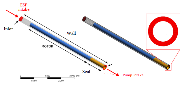
The motor geometry, motor OD, motor length, motor position inside capsule, seal side and position and other relevant parts of the ESP-in-skid were provided by Petrobras SA and Schlumberger’s ESP catalogue for pumping unit series 738 with 750 hp [24]. The final schematic of the ESP is presented in the Figure 2.
![Figure 2: Schematic of the ESP-in-skid capsule and main dimensions. Fluid domain, motor and seal are highlighted. Adapted from Tarcha, et al. [2] and Schlumberger [24].](/fulltextimages/9039/fig_2.png)
The red rectangle depicts the external limits (boundaries) of the fluid domain (volume where the mathematical model was solved). The blue arrow (ESP intake) indicates the gas-liquid mixture inlet boundary and is positioned on the left side of the fluid domain. The red arrow (Pump intake) denotes the fluids outlet boundary located at the fluid domain right side. In the real equipment, this boundary is just before the pump intake. The upper and bottom boundaries are solid walls which models the capsule external casing which is in contact with seawater. The internal boundaries are the motor and seal surfaces.
The blue rectangle (Motor) represents the solid domain. In this domain will be applied the heat conduction model with heat generation. The orange rectangle (Seal) is an adiabatic region and represents the motor seal (motor-pump separator).
The capsule is tilted 5° w.r.t. horizontal plane.
The computational mesh was built with solely hexahedra elements. To simplify the model, the motor and the seal were considered perfect cylinders. This simplification allowed to use a reduced number of elements (390,160) for applying to this geometry 12 radial equally spaced elements in the annular region as shown in Figure 3. The minimal orthogonal quality is 0.7022 and the maximum aspect ratio is 9.67.
The operational points for each case considered for this simulation is summarized in Table 4. The operational point 60 Hz is a single-phase flow because all gas is dissolved in the oil at the ESP intake due to a fluid pressure considered to be above the bubble point, 98 bar, from DeGhetto, et al. [19] correlation. As the motor frequency decreases, the gas volume fraction increases. The 40-60 Hz range of frequencies allowed an extended gas volume fraction effect analysis on the heat transfer.
| Temperature, °C | Pressure, bar | Gas VF, % | ||||
|---|---|---|---|---|---|---|
| 60 | 33.4 | 103.3 | 0.0 | |||
| 55 | 30.4 | 93.6 | 3.5 | |||
| 45 | 27.0 | 68.9 | 17.8 | |||
| 40 | 26.8 | 58.2 | 26.3 |
Table 4: Industrial scale operational points.
The momentum, energy and mass boundary conditions are set based on field data and the heat generated by the motor estimated from Betonico, et al. [25]. A homogeneous mixed oil and gas fluid is considered at the ESP intake. The electrical power converted into heat was not reported for the ESP model in the Betonico, et al. [25] work. For that, the Burt, et al. [26] work was used. The authors suggest that 2% of total electrical power input is converted into heat power. This energy amount was considered to be generated equally in each volume cell inside the motor. The obtained data for each boundary condition and heat source are shown in Table 5.
| Boundary | Variable | Cases | ||||||
|---|---|---|---|---|---|---|---|---|
| 40 Hz | 45 Hz | 55 Hz | 60 Hz | |||||
| Inlet | Oil mass flow (kg/s) | 26.5174 | 30.3841 | 34.1917 | 40.0000 | |||
| Oil flow rate (m³/h) | 100.0 | 114.0 | 127.0 | 150.0 | ||||
| Gas mass flow (kg/s) | 0.53168 | 0.45187 | 0.1207 | 0.0000 | ||||
| Hydraulic Diameter (m) | 0.2734 | 0.2734 | 0.2734 | 0.2734 | ||||
| Turbulence Intensity (%) | 5 | 5 | 5 | 5 | ||||
| Temperature (°C) | 26.8 | 27 | 30,4 | 33.4 | ||||
| Gas Volume Fraction (%) | 26.3 | 17.8 | 3.5 | 0 | ||||
| Outlet | Static Pressure (kPa) | 5820 | 6890 | 9360 | 10330 | |||
| Hydraulic Diameter (m) | 0.0856 | 0.0856 | 0.0856 | 0.0856 | ||||
| Turbulence Intensity (%) | 1 | 1 | 1 | 1 | ||||
| Temperature (°C) | 26.8 | 27 | 30.4 | 38.7 | ||||
| Motor-volume | Heat Source (W/m3) | 17310 | 23280 | 35800 | 52140 | |||
| Seal | Heat Flux (W/m2) | 0 | 0 | 0 | 0 | |||
| External wall | Temperature (°C) | 4 | 4 | 4 | 4 |
Table 5: Industrial scale boundary conditions and heat source.
The oil mass flow is also expressed in oil flow rate (m³/h) because this is the variable (and units) used in field operation. Furthermore, the results of temperature are also presented in function of oil flow rate.
Numerical Approach
A High-Performance Computer (HPC) with 5 nodes (2 quad-core Intel Xeon each) and 32 Gb RAM were used in transient condition simulations.
The SIMPLE (Semi-Implicit Method for Pressure-Linked) pressure-velocity coupling was used. PRESTO! and Second Order Upwind schemes were employed for the pressure and velocity interpolation respectively. To evaluate the variables gradients the Least Squares Cell Based method was applied to each cell. The Second Order Upwind was chosen to obtain the turbulent kinetic energy and the dissipation rate. The Geo-Reconstruct scheme was used to evaluate the volume fraction equation.
For all simulations, the CFL condition was attained. The Courant number is defined by the Equation (17).
| v | ∆t |
|---|
For all cases, two modeling challenges were faced:
- Velocity profiles and flow pattern at the ESP intake domain were unknown;
- Only one pressure point measure was available from the field data, i.e., no pressure drop was available to be compared to the simulation results.
An important numerical strategy issue for this case is the fact that the fluid flow and heat conduction problems have distinct time scales. To overcome that, the following procedure to achieve a global solution was adopted:
- All fluid flow equations with timestep limited by the fluid flow problem (0,01 s for Co = 1) was solved until the fluid mean temperature variation at the pump intake stabilized within 1% (~130 s);
- Then, the fluid flow equations calculations were halted and a larger timestep (10 s, limited by the heat conduction problem) was used until the maximum motor temperature reaches a constant value within 1% margin (~13 h);
- Finally, the fluid flow equations calculations were re- started with the original timestep (Co = 1) until the fluid mean temperature at the at the pump intake stabilized within 1% margin.
- In all cases, the initial condition started from a stabilized fluid condition at 4 °C in all domains (fluid and motor).
Monitoring points were selected to control the simulations and to judge if the solution achieved or not a steady state. The selected monitoring points used were:
- Fluid mean temperature at the pump intake;
- Mean temperature at the motor surface;
- Maximum temperature inside the motor;
- Mean gas volume fraction at the pump intake;
- Gas volume inside fluid domain.
The temperatures calculated from the simulations are then normalized using the Equation (18).
$$ \theta_ {f} = \frac {T}{T _ {i n l e t}} (1 8) $$
f inlet The motor heating dynamics is evaluated using the resulted nondimensional temperature by the Equation (19).
$$ \theta_ {m} = \frac {T - T _ {s e a}}{T _ {\max , m} - T _ {s e a}} \tag {19} $$ sea m m sea max, Where ( ) , @ max m T max T motor domain = , 4 sea T C = ° .
The mean temperature at motor surface is defined by:
$$ T _ {\text {m e a n}, m s} = \frac {1}{A _ {m s}} \sum_ {i = C e l l s} T _ {i}. d A _ {i} \tag {20} $$ Where ms A is the motor surface area, the index i represents the superficial cells of motor external surface, iT is the surface temperature and i dA is the superficial cell area.
Results and Discussion
Motor and Fluids Heating Dynamics
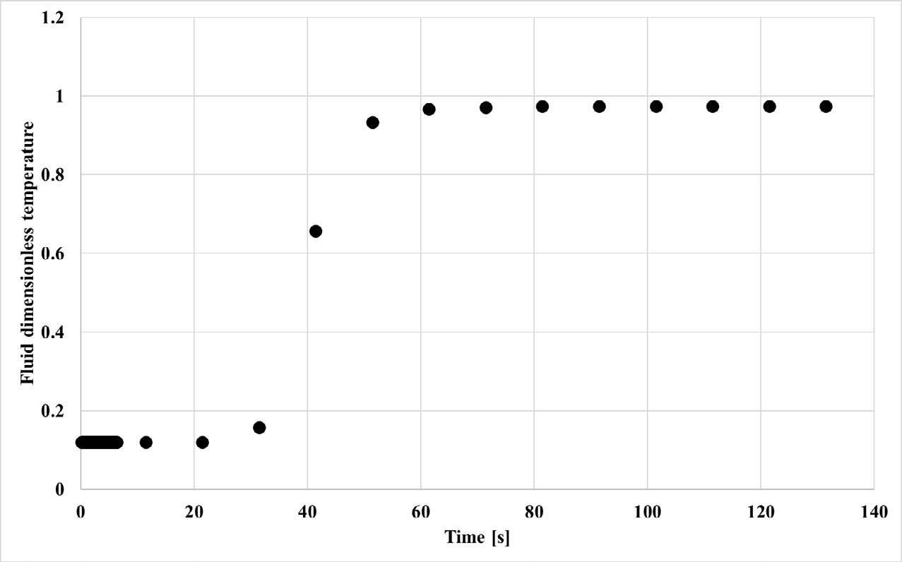
The results presented in this section are the outcome of the first step of the simulation strategy for the 55 Hz case. Similar results are observed for all other cases. The fluid temperature is initially at 4 °C As can be seen in Figure 4, the fluid temperature at the pump intake reaches a constant value ( ) 1 f θ ≈ in 60s (1 minute), whose time delay is due only to the fluid residence time inside the fluid domain volume. During this time, a little increase in the heat transfer occurs between the hot motor and the cold fluid.
After the fluid reaches a constant temperature, the fluid flow equations solving is halted to accelerate the heat conduction in the motor. The motor heating dynamics (Figure
5) is much longer, taking, for the present case, approximately 6 h to reach 95% of the equilibrium temperature. For this reason, the time unit used in this plot is hours.
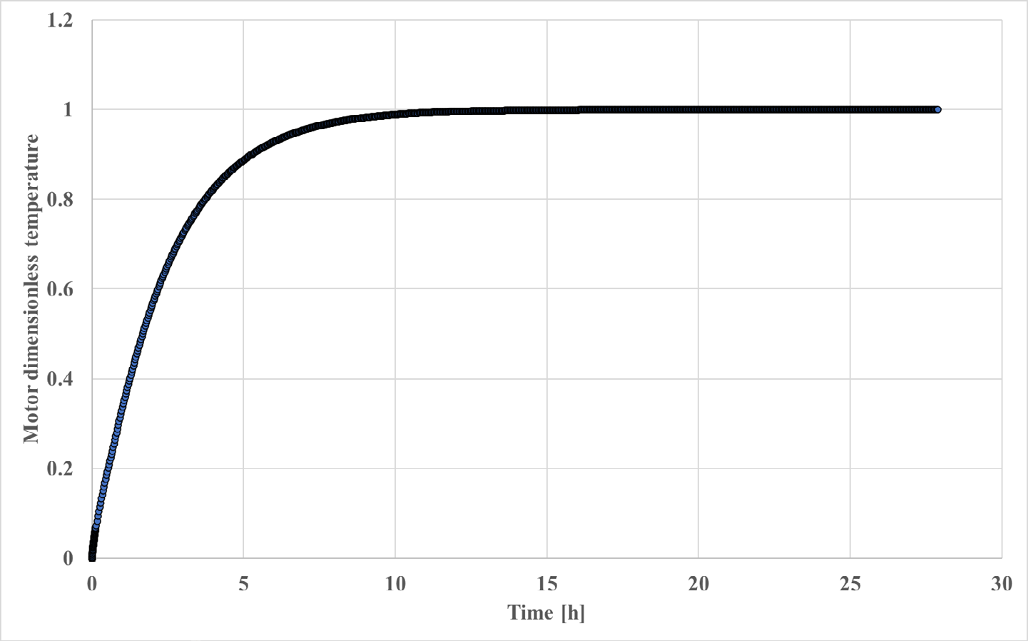
At this point, both the mean motor temperature and the pump intake fluid temperature are stabled but not at the same time. Thus, the next and last step is solving simultaneously both the fluid flow and heat conduction models.
Surface Motor Temperature Field
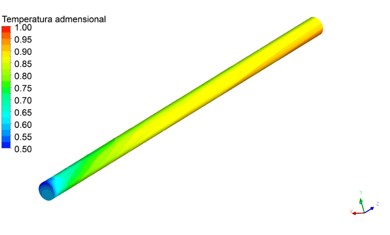
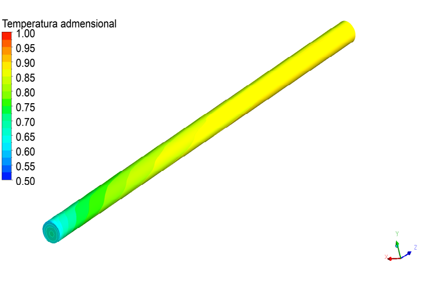
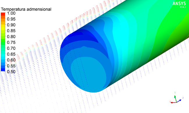
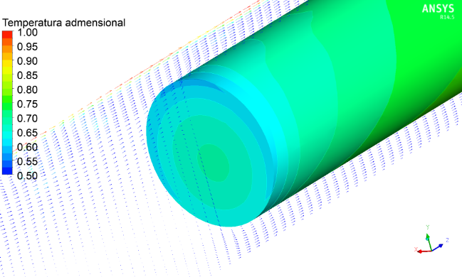
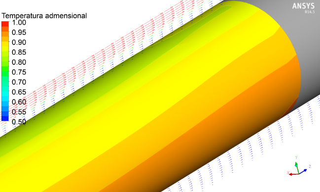
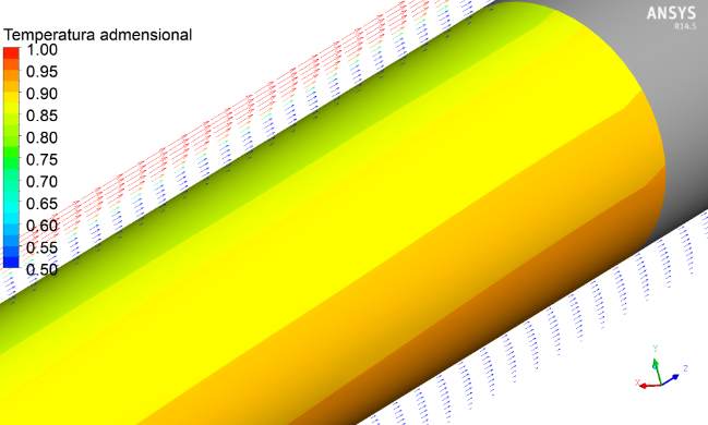
The motor surface temperature fields are shown in the Figure 6 where the fluid is flowing from left to right and the gravity is pointing down. The field values were evaluated using the Equation (19).
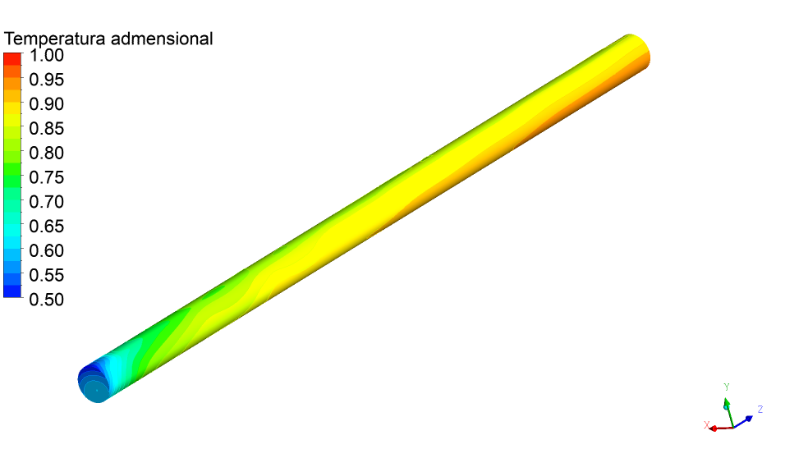
(a) It is possible to notice that the separation of fluids causes a temperature field asymmetry in the two-phase flow cases (Figures 6 (a), (b) and (c)). When only one phase flows, the temperature field is symmetrical (Figures 6 (d)). There is also a temperature increase at the lower region of the motor top near the seal (far right of each graph in Figures 6). It also can be inferred that the turbulent flow instabilities increase the convection at the upper part of the motor bottom (far left of each plot in (Figures 6). This statement is corroborated by observing both the temperature fields and the velocity field plotted together in the Figure 7.
(b)
(c)
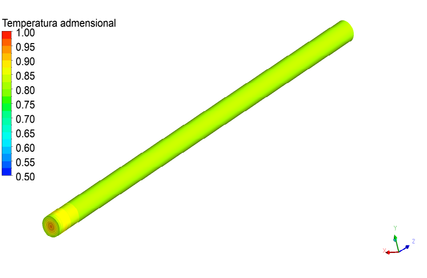
(d) Figure 6: Dimensionless temperature fields on the motor surface at (a) 40 Hz; (b) 45 Hz; (c) 55 Hz; (d) 60 Hz.
(a)
(c)
(b)
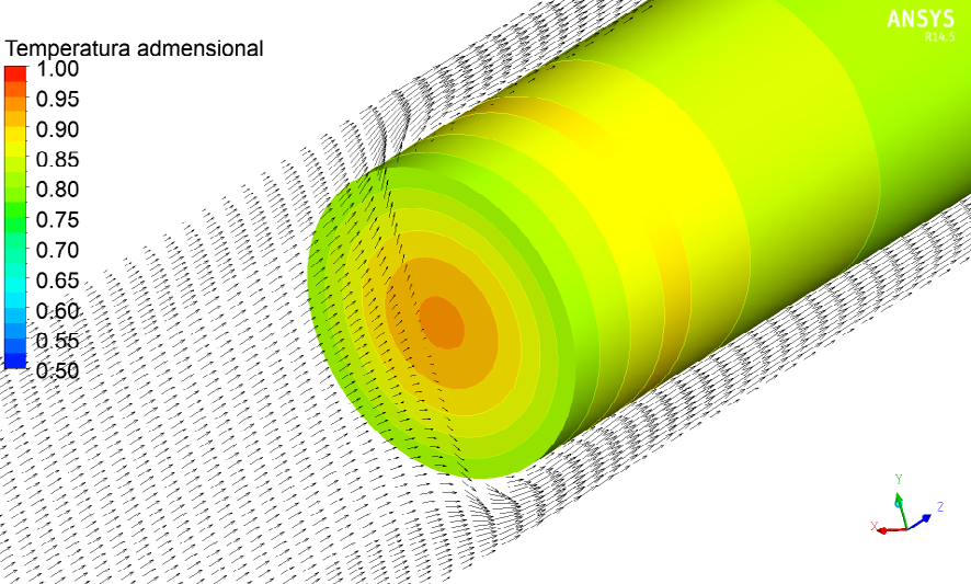
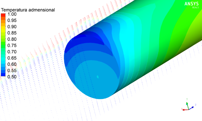
(d) Figure 7: Dimensionless temperature fields on the motor surface and velocity vectors colored by gas volume fraction in a vertical plane: zoom at the motor bottom (inlet). (a) 40 Hz; (b) 45 Hz; (c) 55 Hz; (d) 60 Hz.
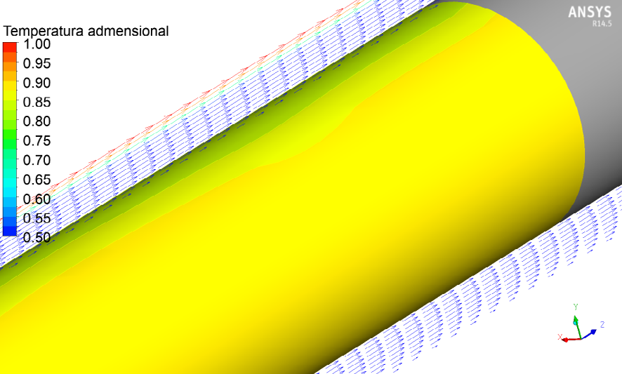
Figure 7 shows the greater the amount of gas, the greater the superficial velocities of the liquid and, consequently, the greater the convection in the upper region of the motor bottom. The single-phase case (d) shows a symmetric field as expected. Figure 8 shows the same fields as shown in the Figure 7, but at the motor top close to the seal.
As observed, the two-phase flow cases (Figure 8 (a), (b) and (c)) present an asymmetric pattern in the vertical direction. As the gas drags the liquid in the upper region, the velocities are greater which makes the convection there to be greater than in the lower region. In the lower speed case (Figure 8 (a) and (b)), a greater difference between the maximum and minimum temperature may be expected.
(a)
©
(b)
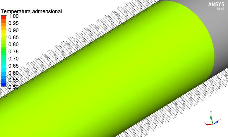
(d) Figure 8: Dimensionless temperature fields on the motor surface and velocity vectors colored associated to the gas volume fraction in vertical plane: motor top (seal). (a) 40 Hz; (b) 45 Hz; (c) 55 Hz; (d) 60 Hz.
Velocity Field Effect on the Motor Surface Temperature
If a velocity profile along a vertical line such as that is observed in the Figure 9 for the 55 Hz case, a quantitative analysis can be made. The velocity behavior is represented by the four lines positioned along the normalized length of the motor (dimensionless ratios of 0.06, 0.30, 0.76 and 0.88). The velocity represented in the Figure 9 plots are normalized by / V V ρ .
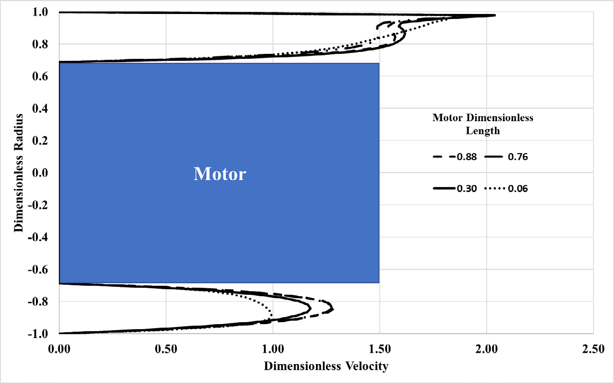
The speed difference between the upper and lower regions is noticeable. As convection is not only related to the speed, if there is solely gas in the upper region, the convection may not be efficient as expected. Figure 10 shows the volume fraction behavior of the gas volume fraction along the same lines of the Figure 9 for this case.
As may be observed, the gas accumulates near the outer motor wall. Therefore, the fluid contact with the motor surface is mainly composed by its liquid phase. For the purpose of a physical analysis, the gas behaves as a shroud liquid accelerator by limiting its available flow area.
Another analysis can be made involving the correlation between the temperature field inside the motor and the fluid around it for the 55 Hz case. This analysis is shown in Figure 11.
In Figure 11 temperature is normalized by the Equation (19). The fluid temperature asymmetry behavior is less clearly observed because the dimensioning scale is much higher (maximum temperature inside the motor). The fluid temperature behavior is characterized by a close sinusoidal shape, related to the characteristic of the double thermal boundary layer formed at the inner wall (motor surface) and outer wall (capsule surface). The maximum temperature calculated for the motor solid domain is close to the seal temperature (at 0.76) due to the seal adiabatic boundary condition.
Finally, Figure 12 shows the results of three characteristic system temperature analysis, including the maximum motor domain temperature.
The higher the flow rate (or, in the present case, the frequency) the greater the heat generated and the maximum motor temperature is greater. On the other hand, the higher the flow rate, the greater the convection, since the difference between the maximum motor domain temperature (Equation (19)) and the mean motor surface temperature increases (Equation (20)). The increase in fluid temperature is not noticeable within the scale used, but it becomes more distinguished as the flow rate increases.
Simulated and Field Measured Thermal Operational Map Comparison
An estimate of the motor temperature as a function of the flow rate or the operational frequency (40 Hz, 45 Hz, 55 Hz, 60 Hz) provided by VSD (Variable Speed Drive) can be made. Figure 13 shows the numerical results, which are coherent with the field data. The results are satisfactory in spite of the uncertainties related to a mean deviation of 5% and to a maximum deviation of 10% in the 60 Hz operational case.
The difference increase between the simulated and field data as the flow rate increases, may be due to the less accurate PVT correlation properties of the related pressure and temperature operational conditions. Also, the arbitrated value for the specific gravity of the gas may be higher than the real ones. The single-phase flow assumption at the highest frequency may provide another explanation for the greater difference, since there may have additional gas in the real operational condition.
Conclusions
The proposed work was to numerically model the turbulent gas-liquid flow with heat exchange around the electric motor of a subsea Skid-ESP system, the adopted methodology was based on the use of CFD tools implemented through the ANSYS Fluent v.15.0 software, and included the employment of specific correlations to describe the oil properties associated with the real oilfield operational data.
The following conclusions may be achieved:
- In spite of the uncertainties related to a mean deviation of 5% and to a maximum deviation of 10% in the 60 Hz operational case, the developed methodology was able to construct a thermal operational map of an ESP-in-skid motor;
- The developed methodology was able to generate coherent dynamic motor’s heating time data around 6 h considering a simplified assumption of a motor made of a homogeneous and isotropic material;
- Instabilities induced by the gas-liquid interface may generate low temperature data at the motor bottom, in the analyzed quasi-horizontal configuration;
- Flow stratification generates high temperatures data at the motor bottom in the region close to the seal;
- The presence of gas, in the quantities provided by DeGhetto (1995), does not favor convection.
Acknowledgement
This work was supported by the Petróleo Brasileiro SA (PETROBRAS).
Nomenclature
| A ms | Motor surface area, m² |
|---|---|
| Co | Courant number |
| c p | Two-phase mixture specific heat, J/kg/K |
| c p,m | Motor specific heat, J/kg/K |
| D ω | ω-equation cross diffusion term, |
| dA i | Surface cell area, m² |
| E | Two-phase mixture specific energy, J/kg |
| G i | Turbulence model equations (i=k or ω) generation terms, m²/s³ |
| g | Gravity acceleration vector, m/s² |
| h | Two-phase mixture specific enthalpy, J/kg |
| k | Two-phase mixture thermal conductivity, W/m/K |
| k ef | Turbulent two-phase mixture thermal conductivity, W/m/K |
| k m | Motor thermal conductivity, W/m/K |
| p | Pressure, bar |
| Pr t | Turbulent thermal Prandtl number |
| Q | Volumetric heat source from the motor, W/m³ |
| T | Two-phase mixture Temperature, °C |
| T ref | Reference temperature, °C |
| T inlet | Two-phase mixture temperature at inlet, °C |
| T sea | Sea temperature, ºC |
| T max,m | Motor maximum temperature, °C |
| T mean,ms | Motor surface mean temperature, °C |
| t | Time, s |
| v | Two-phase mixture velocity vector, m/s |
| v | Velocity magnitude, m/s |
| Y i | Turbulence model equations (i=k or ω) dissipation terms, m²/s³ |
| α g | Gas volume fraction |
| α l | Liquid volume fraction |
| ρ | Two-phase mixture density, kg/m³ |
| ρ g | Gas density, kg/m³ |
| ρ l | Liquid density, kg/m³ |
| ρ m | Motor density, kg/m³ |
| µ | Effective viscosity, Pa s |
| µ m | Two-phase mixture viscosity, Pa s |
| µ g | Gas viscosity, Pa s |
| µ l | Liquid viscosity, Pa s |
| µ t | Turbulent viscosity, Pa s |
| k | Turbulent kinetic energy, m²/s² |
| Γ i | Turbulence model equations (i=k or ω) diffusivities, m²/s |
| ω | Turbulent kinetic energy dissipation frequency, 1/s |
| σ i | Turbulent Prandtl number (i=k or ω) |
| ∆x | Equivalent control volume size, m |
| ∆t | Timestep, s |
| θ f | Dimensionless two-phase mixture temperature, |
| θ m | Dimensionless motor temperature, |
References
-
Viana AM, Manzela AA (2015) Avanços e Desafios em Sistemas de Bombeio Centrífugo Submerso. Revista de Engenharias da Faculdade Salesiana 2: 26-32.
-
Tarcha BA, Borges OC, Furtado RG (2015) ESP Installed in a Subsea Skid at Jubarte Field. SPE Artificial Lift Conference, Latin America and Caribbean.
-
Urban A, Boechat N, Haaheim S, Sleight N, Debacker I, et al. (2015) MOBO ESP Interventions. OTC Brasil, Rio de Janeiro, Brazil.
-
Roberto MAR, Oliveira PS, Pyramo BM (2013) Mudline ESP: Electrical Submersible Pump Installed in a Subsea Skid_._ Offshore Technology Conference.
-
Takacs G (2009) Electrical submersible pumps manual: design, operations, and maintenance.
-
Ofuchi EM, Stel H, Vieira TS, Ponce FJ, Chiva S, et al. (2017) Study of the effect of viscosity on the head and flow rate degradation in different multistage electric submersible pumps using dimensional analysis. J Pet Sci Eng 156: 442-450.
-
Deshmukh D, Samad A (2019) CFD-based analysis for finding critical wall roughness on centrifugal pump at design and off-design conditions. J Braz Soc Mech Sci Eng 41: 58.
-
Peng L, Wang Y, Yan F, Nie C, Ouyang X, et al. (2020) Effects of Fluid Viscosity and Two-Phase Flow on Performance of ESP. Energies 13(20): 5486.
-
Rodrigues JD, Finaish F, Dunn-Norman S (2000) Parametric study of motor/shroud heat transfer performance in an electrical submersible pump (ESP). J Energy Resour Technol Sep 122(3): 136-141.
-
O’Bryan R, Rutter R, Sheth K (2012) Validation and Optimization of Heat Transfer in The Electrical Submersible Pump Motor By CFD. ASME International Mechanical Engineering Congress and Exposition 6: 955-961.
-
Lin RY, Shao CB, Li J (2013) Study on two-phase flow and heat transfer in offshore wells. J Petrol Sci Eng 111: 42- 49.
-
Betônico GC (2013) Study of temperature distribution on ESP motors. Master’s Thesis, Faculty of Mechanical Engineering, Unicamp.
-
Martins JR, Ribeiro DC, Pereira FAR, Ribeiro MP, Romero, et al. (2020) Heat dissipation of the Electrical Submersible Pump (ESP) installed in a subsea skid. Oil & Gas Sci Technol-Rev IFP Energies nouvelles 75(13).
-
Versteeg HK, Malalasekera W (2007) An Introduction to Computational Fluid Dynamics: 2nd (Edn.), The Finite Volume Method.
-
Xu JH, Li SW, Tan J, Luo GS (2008) Correlations of droplet formation in T-junction microfluidic devices: from squeezing to dripping. Microfluid Nanofluid 5: 711-717.
-
Menter FR (1994) Two-Equation Eddy-Viscosity Turbulence Models for Engineering Applications. AIAA Journal 32(8): 1598-1605.
-
Bradshaw P, Ferriss DH, Atwell NP (1967) Calculation of boundary layer development using the turbulent energy equations. J Fluid Mech 28(3): 593-616.
-
Fluent (2013) ANSYS Fluent Theory Guide v15.0.
-
De Ghetto G, Paone F, Villa M (1995) Pressure-Volume- Temperature Correlations for Heavy and Extra Heavy Oils. International Heavy Oil Symposium, Society of Petroleum Engineers, Calgary, pp: 647–662.
-
NIST (National Institute of Standards and Technology) (2018) Chemistry web book.
-
Gambill WR (1957) You Can Predict Heat Capacities. Chem Eng 64(6): 243-248.
-
Moshfeghian M (2011) Development of a New Generalized Correlation for Natural Gas Heat Capacity. 90th Annual GPA Convention, San Antonio, Texas, USA.
-
Cragoe CS (1929) Thermal Properties of Petroleum Products. NBS Miscellaneous Publication No. 97, US Bureau of Standards.
-
Schlumberger (2017) REDA Electric Submersible Pump Systems Technology Catalog, Houston.
-
Betonico GC, Bannwart AC, Ganzarolli MM (2015) Determination of the temperature distribution of ESP motors under variable conditions of flow rate and loading. J Petrol Sci Eng 129: 110-120.
-
Burt C, Piao X, Gaudi F, Busch B, Taufik NFN, et al. (2006) Electric motor efficiency under variable frequencies and loads. ITRC report R-06-004.
- Nigeria’s Vulnerability in the Face of Global Energy Policy
- A Simulation Study of Investigation of Optimum Oil Production Performance by Applying Various Gas Injection Methods in Oil Reservoir
- Characterization of Permo-Triassic Reservoirs through Thermal Maturity Assessment of Westphalian Source Rocks in the Cheshire Basin
- Influence of Microwax on the Rheological and Thermal Behaviour of a Wax Crude Oil
- Real-Time Monitoring and Performance Optimization of Steam Injection in Heavy Oil Reservoirs Using Fiber Optic Sensing and Integrated Predictive Simulation Models
- Rapid On-Site Determination of the Total Petroleum Hydrocarbon Content of Soils by Handheld Fourier Transform Near-Infrared Spectroscopy: Development of a Global, Site- and Scanner- Independent Calibration Model