Stress Analysis of Pipe-In-Pipe Systems under Free Span for Deep Water Pipeline Applications
This study examined the phenomena of free span for a pipe -in- pipe (PIP) system for pipeline application. Two different span length of 8 and 30 meters are modelled and simulated using nonlinear stress analysis. The effect of pressure, temperature and gravity on the PIP system are determined and compared with conventional single pipeline. From the results obtained, it is clear that the finite element analysis (FEA) results correlated very well with those calculated using analytical methods. Percentage differences were generally less than 10%, with some discrepancies which were due to assumption of thin-walled theory which assumes a radial stress equals to zero, whereas the FEA calculates a non- zero radial stress. The key finding in this study demonstrated the strong potentials of PIP system in terms of structural reliability for deepwater pipeline application. Specifically, the 30m single pipe in free span (with pressure and temperature) deflected 205.1mm, more than double the corresponding PIP. This knowledge can be beneficial to selection and design considerations for pipeline system responses to both the gravity, thermal and pressure loading as well as the potential failure modes that may results in a typical scenario. Various theoretical calculations of stresses are used to validate the finding in this study of the single pipe and PIP models for flat seabed and free span.
Introduction
Hydrocarbon production from offshore fields has been accomplished since the 1970s using platforms and subsea tiebacks. In more recent years, this technology has enabled deeper waters to be explored, giving access to previously impractical and uneconomic reservoirs. However, subsea separation, gathering and exporting the produced fluids to shore from deep water is challenging. Pipeline system remains the safest and economically viable means of mitigating the transportation challenges of oil and gas resources to shores from these challenging locations such as deep-water [1, 2].
However, deep-water fields development presents specific challenges to pipeline design, construction, installation, operation and maintenance [3, 4, 5, 6]. For example, El-Chayeb, et al. [7]; Furnes and Berntsen [8]; present pipeline crossings to cause problems such as on-bottom hydrodynamic instability and Vortex Induced Vibration (VIV). However, recently the study of Nikoo, et al. [9] and Bi and Hao [10] demonstrated the effectiveness of PIP in mitigating the VIV challenge for subsea pipeline. Bruton, et al. [11] pointed out that a key design challenge for deep- water pipelines is to control the thermally induced lateral buckling, which usually involves large lateral displacements of the pipeline at different locations.
PIP and pipes with high strength capacity are currently seen as the optimum choice for the development of deep-water oil and gas fields such as high-pressure high temperature fields – HPHT [12]. This is because PIP system can provide the desired thermal insulation and structural integrity for the transportation of the produced fluids from deep-water to shores regardless of the sea condition. Furthermore, PIP systems are capable of maintaining the produced hydrocarbons at temperatures well above 120°C and pressures in excess of 10,000psi [13]. Another study by Reis, et al. [2] on the dynamic response of free pipelines proposed linear stability analysis (LSA) as an alternative to approximate analytical methods capable of providing accurate solutions to complex problems.
Of importance is the free span scenario which relate to an unsupported length on a structure analogous to the classic beam bending scenario explored in fundamental statics. A pipeline free span occurs between two shoulders on the seabed as shown in Figure 1. The phenomenon of pipeline free span is where a pipeline has an unsupported length. This may occur on the seabed where a section of softer sand has been washed away from underneath the pipeline due to sea currents. When pipelines are installed on the seabed there is a key focus on ensuring they are as safe as possible to other users, especially trawling vessels [14]. Free spans are inevitable for unburied pipelines as a result of uneven seabed and local scouring resulting from flow turbulence and instability [15].
![Figure 1: The phenomenon of pipeline free span is where a pipeline has an unsupported length. This may occur on the seabed where a section of softer sand has been washed away from underneath the pipeline due to sea currents. When pipelines are installed on the seabed there is a key focus on ensuring they are as safe as possible to other users, especially trawling vessels [14]. Free spans are inevitable for unburied pipelines as a result of uneven seabed and local scouring resulting from flow turbulence and instability [15].](/fulltextimages/9732/fig_1.png)
There are a number of effects and dangers of a pipeline in free span, the most obvious danger is the interaction with trawling gear becoming caught underneath the span. There are regulations set out in Det Norske Veritas (DNV)-RP-F111 on interference between trawl gear and pipelines regarding the maximum acceptable height and length of free spans. Even though trawl gear hooking and getting stuck on pipelines is a rarity, free spanning pipelines are the most common causes of hooking [16]. DNV-RP-F111 [11] covers the effect of trawling gear interaction with free spanning pipelines and discusses the calculation of the critical height of free spans. In addition, over the length of the free span the pipeline would experience bending forces through the unsupported weight of the pipe, these forces would be exacerbated by the effects of temperature and pressure within the pipeline [17, 18].
A pipeline in free span will experience increased stresses due to bending stresses caused by the weight of the pipeline, which are added to the already present stresses from pressure and temperature (from both the hydrocarbon inside the pipeline and the seawater outside the pipeline). These potentially increased stresses need to be considered at the design stage otherwise the pipeline may fail [19].
Vortex Induced Vibration, or VIV, is a primary cause of fatigue damage on free spanning sections of a pipeline [20]. VIV is caused by vortex shredding caused by currents flowing over the pipeline. When a current flow normal to a pipeline free span, vortices shred and thus a periodic wake is created [20]. This alters the local pressure and results in the alteration of the forces generated, at the frequency of vortex shredding [20]. Should the current be sufficiently strong, the frequency of the oscillations may be near, or match the natural frequency of that pipeline. If this is the case, and the resonant oscillations and cyclic stress are both large enough and of sufficiently frequent occurrence, long term fatigue damage can occur which can jeopardise the safe operation of that pipeline [20]. The natural frequency is a function of the span length and therefore the maximum allowable span length, in terms of fatigue control, may be determined [20]. DNV-RP-F105 [21] details out combined wave and current loading on free spans, interested readers are referred to this recommended practice.
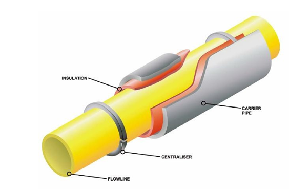
Historically, the first known PIP system installed was by Pertamina Offshore Indonesia in 1973 [1]. It was 8 miles long with an outer diameter of 40 inches and an inner diameter of 36 inches [1]. A typical PIP set up can be seen below in Figure 2. The yellow flowline is wrapped in red insulation and the carrier or jacket pipe is labelled in grey, this set up also uses centralisers as shown. Centralisers are used to ensure the non-load- bearing-insulation does not become compressed between the jacket pipe and flow line.
A very well-engineered PIP system can prevent wax and hydrate formations due to cooling along the length of the pipeline. Hydrates are ice-like crystals that form where there is high pressure and low temperature, thus maintaining the temperature of the well fluids above the hydrate formation temperature would be essential to ensure the flow of hydrocarbons. In addition, while the PIP is serving this function, it is also expected to resist all potential forces and loads that may undermine the system structural integrity. This is advantageous as otherwise costly intervention may be required if the production rate notably decreases. Literature has shown that the safe operating life of a pipeline depends on two main factors. Primarily on the stress levels present during installation, testing and operation [23, 24]. Secondly on the proper determination and control of fatigue damage, which is primarily caused by the cyclic loading of free spans by steady-state or cyclic current conditions [20].
Therefore, there is an urgent requirement for a pipeline system with low thermal conductivity and meeting the structural integrity requirement in a stormy deep-water location. PIP systems can provide this using high insulating material (thermal foams) sandwiched between two pipes and its outstanding structural responses established through simulation. Specifically, this study examined stresses and displacements in the PIP system under free span situation. This is crucial in establishing the possible failure modes of the PIP system; since its structural integrity is a key requirement at both installation and operation phases as noted above.
Heat Transfer Coefficients of Different Pipeline System
A Pipe-in-Pipe (PIP) system employs a highly insulating material (thermal foams) sandwiched between two pipes to achieve a low thermal conductivity. This would help to maintain the fluids temperature in the carrier pipe mitigating the formation of any flow assurance issues such as wax and hydrates. PIP systems are made up of two concentric pipes. An inner pipe is inserted into a larger diameter outer pipe with insulation material often contained within the annulus. The inner pipe carries the fluids being transported whilst the outer pipe provides protection from water penetration and the external hydrostatic pressure. Installing a second pipe around the product pipeline isolates the carrier pipeline from the cold seawater, this also creates a space that can be filled with a low heat transfer coefficient (U-value) material. PIP systems can provide a U- value of 2 (W/m2K) or less.
PIP systems are employed when a low heat transfer coefficient (U-value) is required. Typically PIP systems can provide a U-value of 2.0 W/m2K or less as shown in Figure 3. However, it could be expected that PIP or bundle type systems would be capable of providing U-values of less than 1.0 W/m2K [25]. The requirement for such a low U- value may occur where flow assurance issues such as hydrates would threaten the production rate through the pipeline.
Figure 3 shows the effectiveness of PIP systems in achieving low heat transfer coefficients, especially in deep- water. As there are various components in PIP systems, they can be specifically designed for each field’s unique requirement. This could include changing the gap thickness between the inner and outer pipes to optimize insulation capabilities or by using more centralizers to improve structural stability. Single pipelines with a small outer diameter, normally 16 inches or less usually have to be trenched and/or buried which is an extremely expensive process. However due to the added weight and extra mechanical protection from the outer pipe there is less need for the PIP to be laid in a trench or buried.
![Figure 3: However, it could be expected that PIP or bundle type systems would be capable of providing U-values of less than 1.0 W/m2K [25]. The requirement for such a low U- value may occur where flow assurance issues such as hydrates would threaten the production rate through the pipeline.](/fulltextimages/9732/fig_3.png)
Governing Equations
In both theory and practice, Harrison, et al. [27] established that the hoop stress in the carrier (inner) pipe, $\sigma_{hc}$ was evaluated using equation (1). Similarly, the hoop stress in the jacket (outer) pipe, $\delta_{hj}$, is calculated using equation (2). These calculations are simplified by the assumption that there is a degree of separation between the jacket and carrier pipes, therefore the only pressure acting on the jacket pipe is the external (hydrostatic) pressure and the only pressure acting on the carrier pipe is the internal pressure.
$$\sigma_{hc} = \frac{P_i D_c}{2 t_c}$$ \hspace{1cm} (1)
Where, $P_i$ is the internal operating pressure $D_c$ is the outer diameter of the carrier (inner) pipe $t_c$ is the wall thickness of the carrier (inner) pipe
$$\sigma_{hcj} = \frac{P_i D_j}{2 t_j}$$ \hspace{1cm} (2)
Where, $P_j$ is the external hydrostatic pressure $D_j$ is the outer diameter of the jacket (outer) pipe $t_j$ is the wall thickness of the jacket (outer) pipe
Harrison, et al. [28] pointed out that a pipeline is associated with an active section and a fully restrained section whether surface or buried. The determination of the active length or anchor length of the pipeline is crucial for the design and operation of the pipeline. The active length depends on the length of the pipeline. In a relatively short pipeline, for example, the entire length may be active. The section of the pipeline in the anchor region is not subject to either axial elongation or, axial friction with the seabed [28]. Pipeline burial results in a larger contact area with the soil and hence, a greater amount of friction and soil pressure. This limits the pipeline’s potential for movement and expansion [27]. However, due to the cost implication of pipeline burial, it is often more cost effective to leave the pipeline unburied, especially in deep water [27, 29]. The contact area for the unburied pipeline is relatively low, which results in potentially larger longitudinal and lateral deviation or buckling [26, 30].
The following formulae are relevant to a pipeline which is assumed to have a uniform temperature along its length [28]. In order to solve equation (3) it is first necessary to determine the reduced seabed friction coefficient; the forces due to thermal effects; forces due to Poisson’s effects; the spool piece friction force and the end cap force. The seabed friction is altered by the spacer friction. Spacer friction causes a compressive distributed load on the inner pipe. There is also a tensile force which affects the seabed friction coefficient. This reduced seabed friction coefficient, $\mu_o$, is calculated using (3) after Bokaian [28].
$$\mu_o = \mu \left( 1 - \frac{\mu_s}{w_s} \frac{\mu}{w_{pip}} \right)$$ \hspace{1cm} (3)
The thermal force on the inner pipe, NTc, is evaluated using equation (4) [28].
$$N_{TC} = E_p A_{SC} \alpha \left( T_i - T_a \right)$$ \hspace{1cm} (4)
Where, $E_p$ is the Young’s Modulus of the inner pipe. $A_{SC}$ is the steel cross-sectional area of the inner pipe. $\alpha$ is the thermal expansion coefficient for the steel. $T_i$ is the design temperature of the inner pipe. $T_a$ is the ambient temperature which is assumed equal to the installation temperature.
Expression (5) is used to determine the force on the inner pipe due to Poisson’s effects, Nvc [28].
$$N_{vc} = \sigma_{hc} A_{sc} V$$ \hspace{1cm} (5)
The end cap force on the bulkhead is evaluated from the relationship shown in equation (6) [28].
$$N_E = \left( P_i A_i \right) + \left( P_{ans} A_{ans} \right) - \left( P_j A_{ij} \right)$$ \hspace{1cm} (6)
Where, $P_i$ is the inner pipe design pressure $A_{sc}$ is the inner area of the inner pipe $P_{ans}$ is the pressure in the annulus which is equal to atmospheric pressure $A_{ans}$ is the annular area between the inner and outer pipes $P_j$ is the external hydrostatic pressure $A_{oj}$ is the outer area of the outer pipe.
The proportion of the end cap force acting on the inner pipe, NEc, is determined using equation (7) [28].
$$N_{EC} = \frac{E_p A_{sc}}{E_p A_{sc} + E_c A_{sj}} N_E$$ \hspace{1cm} (7)
Where, $E_c$ is the Young’s modulus of the outer pipe $A_{sj}$ is the steel cross-sectional area of the outer pipe
The end cap strain, $\varepsilon_{gt}$, is calculated using equation (8) [28].
$$\varepsilon_{gt} = \alpha \left( T_{dj} - T_a \right)$$ \hspace{1cm} (9)
Consequently, the force on the outer pipe due to thermal effects, NTj is calculated using equation (10) [28].
However, it is possible to determine the sum of the thermal effects on the pipeline using equation (12) [28].
$$\sum N_T = N_{tc} + N_{j}$$
The sum of the forces due to Poisson’s effects may be calculated using equation (12) [27].
$$\sum N_v = N_{vc} - N_{j}$$
The pipeline was assumed to have two identical tie-in spool pieces at the two ends. Thus, there is a static point at the centre of the pipeline, which is also located at the centres of the models in current analyses [28]. Therefore, due to force equilibrium, equation (13) may be solved for the active length. It should be noted that this active length occurs in long pipelines, as friction with the seabed limits the longitudinal extension of the pipeline.
$$L_a = \frac{L}{2} \left( \frac{\mu_S w_c L_{sc}}{2} \sum N_v + N_E - F_S}{\mu_0 L W_{pip}} \frac{E_c A_{sc}}{E_p A_{sc}}$$
Where, $L_a$ is the active length of the pipeline $\mu_s$ is the spacer friction coefficient $W_c$ is the weight of the carrier pipe in air $F_s$ is the tie-in spool piece friction force
in order for equation (13) to be valid, the following criteria must be met:
- The active length must be within $0 < L_a \leq L/2$
- In terms of tie-in spool piece friction force,
- $$F_s \leq \sum N_T - \frac{\mu_s W_{sc}}{2} \left| -\sum N_v + N_E \right|$$
- The limit length between short and long pipes, $L_0$ must be $\geq L_0$
Where $L_0$ is defined by equation 14.
$$L_0 = \frac{1}{\mu_o w_{pip}} \left( \frac{E_c A_{sc}}{E_p A_{sc}} \right) \left( -\sum N_T - \sum N_v + N_E - F_s \right)$$
It should be noted that if $L_o < L$, the pipeline is deemed to be short, as such the entire pipeline is deemed to be active, and longitudinal seabed friction acts along that pipeline entire length [28].
With the active length of the pipeline known, it is possible to determine the longitudinal stress within the carrier and jacket pipes. The relevant formula to use is determined by the relationship between the active length and the distance of interest along the pipe, $x$. In the case of $x \geq Lac$, as is the case in the models in the current analyses, (15) may be used to calculate the longitudinal (axial) stress in the carrier (inner) pipe, $olc$, and (16) may be used to calculate the longitudinal stress in the jacket (outer) pipe, $olj$ [27].
$$\sigma_{ic} = -\alpha E \Delta T_x = v \frac{P_i D_c}{2_{rc}}$$
Where, $\Delta T_x$ is the temperature distribution at $x$ distance from the inlet and is determined using:
$$\sigma_{ij} = v \frac{P_j D_j}{2_{j}}$$
The temperature distribution at $x$ distance from the inlet may be calculated using expression below presented by Harrison, et al. [27].
$$\Delta T_x = \left( T_i - T_e \right) e^{-K_2 x}$$
Where, $K_2$ is the overall heat transfer coefficient [27]. However, in the case of the $x < Lac$ (18) and (19) must be used in order to determine the longitudinal stresses in the carrier and jacket pipes respectively [27].
$$\sigma_{ic} = \frac{P_i A_{ic}}{A_{sc}} - \frac{f_c W_{cs}}{A_{sc}} - \frac{F}{A_{sc}}$$
Where, $F$ is the equilibrium force in the carrier and jacket pipes respectively
$$\sigma_{ij} = \frac{f}{A_{ij}} - \frac{f_j W_{cs}}{A_{ij}} + \frac{P_j A_{ij}}{A_{ij}} - \frac{f_i W_{js}}{A_{ij}}$$
The von-Mises stresses in the carrier and jacket pipe may be evaluated separately using Equation 21 in the carrier pipe, $\sigma_{vmc}$, and equation (22) in the jacket pipe, $\sigma_{vmj}$.
$$\sigma_{vmc} = \sqrt{\frac{1}{2} \left( \sigma_hc - \sigma_{ic} \right)^2 + \left( \sigma_{ic} - \sigma_{R} \right)^2}$$
$$\sigma_{vmj} = \sqrt{\frac{1}{2} \left( \sigma_hj - \sigma_{ij} \right)^2 + \left( \sigma_{ij} - \sigma_{R} \right)^2}$$
Modelling and Simulations
The modelling of the PIP system, including the inner and outer pipes and the insulation, were created using Solidworks CAD software. These were created by first using the sketch tool to sketch half of each pipe (due to the half symmetry used in the FEA). These sketches were then extruded, thus creating each part. After each part was created, the PIP system was mated into an assembly and important into the FEA model as a .STEP file, which is a widely accepted file type for both CAD and FEA geometries. Unintentional gaps generated between components, which can affect the analysis. However, these can be adjusted using the Interface Treatment settings in ANSYS Workbench.
The dimensions of the PIP pipeline, including the inner/ outer pipe and insulation material are shown in Table 1. Half symmetry is used in the analysis in order to improve computational efficiency.
| Outer Diameter (mm) | Inner Diameter (mm) | Wall Thickness (mm) | D/t Ratio | |
|---|---|---|---|---|
| Outer (Jacket) Pipe | 406.60 | 362.90 | 21.85 | 18.6 |
| Insulation Material | 362.90 | 304.80 | 29.05 | 12.49 |
| Inner (Carrier) Pipe | 304.80 | 269.80 | 17.50 | 17.42 |
Table 1: PIP geometrical dimensions.
The dimensions used for the seabed are shown in Figure 4 for the flat seabed PIP under a 4-meter free span. The thickness used for the seabed in this analysis is 2mm, in order to ensure correct contact as the analysis is three dimensional.
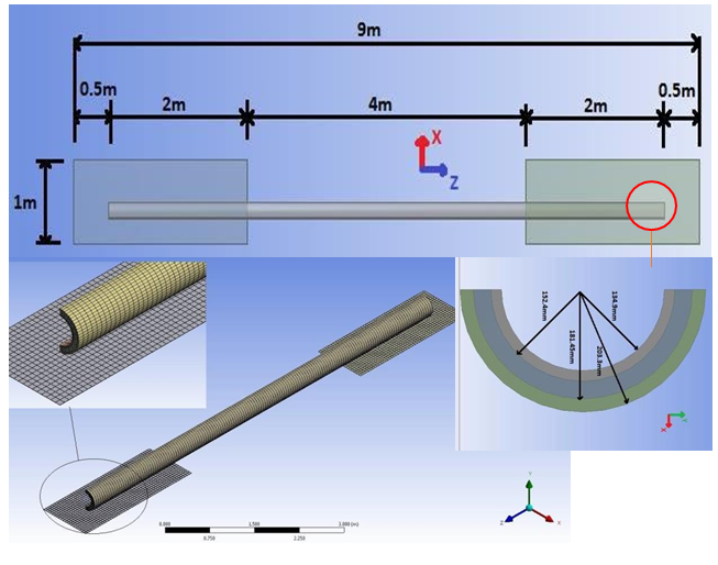
In order to ensure successful analysis, the model is constrained in the X, Y and Z axes. The constraints used are as follows: Z-Axis correspond to the pipeline longitude. A 0 displacement (Z axis = 0) was applied to the end faces of the pipeline. This is because the modelled section is only one short section of the much larger pipeline and therefore the overall pipeline would constrain the movement of the short section. Pipeline Y-Axis (Vertical Radial)/Seabed: A remote displacement was applied to the face(s) of the seabed which are fixed in all directions, including rotational, providing the Y axis constraint for the pipeline also. Pipeline X-Axis (Horizontal Radial): A symmetry region provides the X-axis constraint which was applied to the cut off of the half symmetry model.
Pressure loads are applied in the static structural analysis system in ANSYS Workbench. This consists of: Internal operating pressure of 64.13 MPa (9.3ksi) applied to the inner faces of the pipeline. External hydrostatic pressure of 14.48 MPa (2.1ksi) applied to the outer faces, which corresponds to a depth of 4700ft.
In order to solve non-linear static models, ANSYS uses the Newton- Raphson approach. This is an iterative procedure which determines the out- of balance load vector. The program then performs a linear solution, checks for convergence and repeats until convergence is achieved.
Contact problems considering frictional contact may be split into two types, concave and convex. The contact between the pipes and the insulation may be said to be concave, as the 2 two pipes fit closely together without deformation in both cases [31]. However, the contact between the pipe and seabed may be said to be convex, as the components have dissimilar profiles. All contact problems are highly non-linear and hence require an iterative solution. As such, Surface-to- surface contact is used in this analysis.
Results and Discussion
Pipe-In-Pipe systems are being chosen as they offer advantages over single pipelines. The most important advantage is the much-improved thermal management. Single pipelines require many thermal coatings and wet insulation to be wrapped around the outside of the pipeline;
however, these have been found to work poorly in HPHT fields [26].
The use of PIP systems to transport fluids from deep water HPHT fields ensures that the hydrocarbons reach its desired destination at the required temperature, well above the temperature needed for wax and hydrates to form. Another major advantage of PIP over the conventional single pipe is its structural reliability. PIP system reduced the deflection in free spans by over 50% in similar conventional single pipe. In general, regardless of the situation, when it comes to deep water pipeline PIP proved to be a better option than the conventional single pipeline despite the higher initial costs.
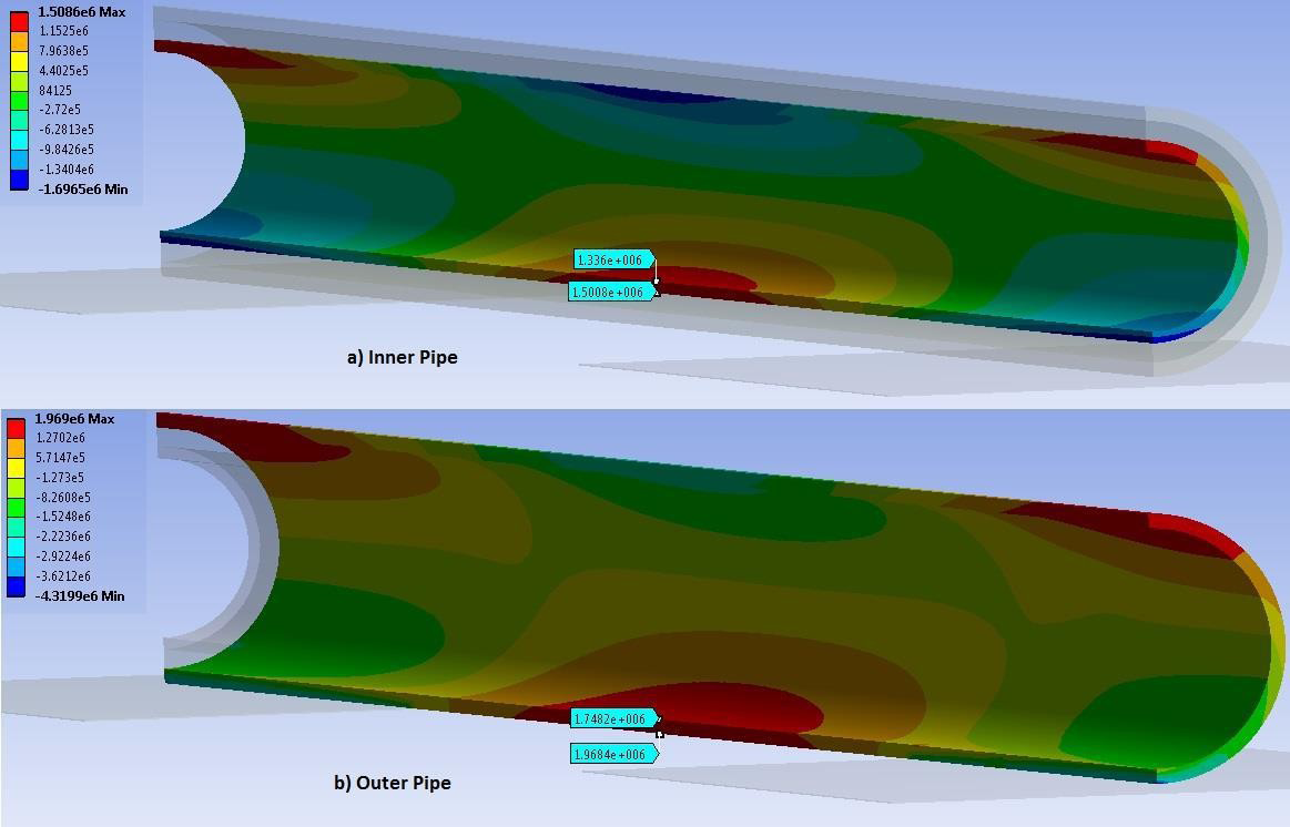
In order to investigate the effect of free span two different span length are modelled, simulated and the results presented. The first is 8m free span length. This model is solved to determine the axial stress and Y-axis deformation on both the inner and outer pipes. As it can be seen by the legend on this Figure (5a); maximum and minimum stresses are 1.509MPa and -1.697MPa respectively. However, the bending stresses are shown by the data labels and are 1.336MPa at the inner radius and 1.501MPa at the outer radius. The outer pipe is shown by Figure (5b). Using probe tool, the bending stresses are 1.748MPa on the inner surface and 1.968MPa on the outer surface.
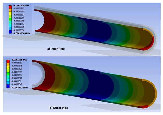
By solving the model for the Y axis deformation, the maximum deflection due to bending is computed. The inner pipe deflects a maximum of 0.3756mm and the outer pipe
0.3753mm. This is shown by the dark blue contours or bands in a) and b) of Figure 6. These deflections occur at the midpoint of the PIP system.
However, a comparison is made between the simply supported and the FEA to evaluate the bending stress obtained using the two approaches for validation purpose. Table 2 summarizes the results of both the inner pipe and outer pipe.
| Bending Stress (MPa) | |||
|---|---|---|---|
| Theory: Simply | FEA | ||
| Inner Pipe | Inner Radius | 0.815 | 1.336 |
| Outer Radius | 0.92 | 1.501 | |
| Outer Pipe | Inner Radius | 1.096 | 1.748 |
| Outer Radius | 1.228 | 1.968 |
Table 2: bending stress comparison between theory and FEA.
However, as it can be seen on the FEA results, stress has been found to be approximately 0.5MPa larger than the simply supported bending stress. One factor that could be causing discrepancies between the predicted and actual results is the percentage of the model that is in free span. Only half of the short model is in free span, which means the other 4 metres, 2m each side is still being constrained (by the rigid seabed and the Z-axis displacement being set to zero). This 2-metre gap between the fixed and the simply supported (edge of the seabed) constraint could have an influence on the bending stresses causing them to be greater than expected. This phenomenon is unlikely to cause any issues in the offshore pipeline since the bending stress and displacement exhibited are too small to cause any issue to the system, either locally or globally. This can be seen by the deformation of both pipes Figure 6 as they each deflect less than a millimetre.
Effect of Pressure on the PIP System Under Free Span
In order to study the effect of pressure on the PIP system, extra loading conditions were applied alongside gravity. An internal and external pressure was applied to the inner surface of the inner pipe and the outer surface of the outer pipe. These pressures were 64.12MPa and 14.47MPa respectively.
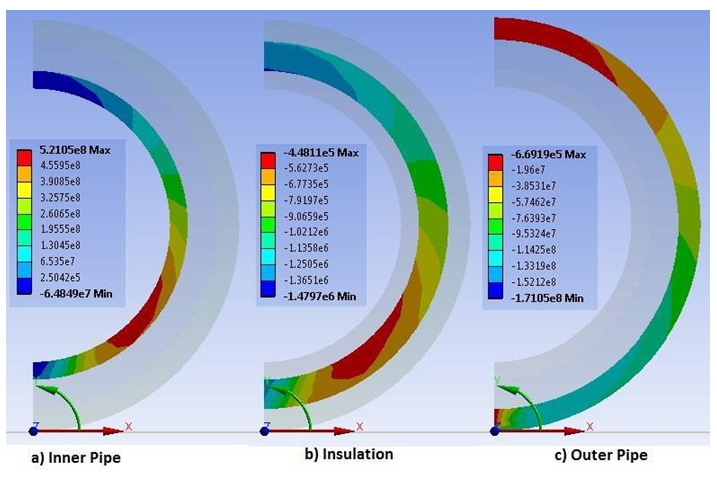
This model was solved to determine the von Mises, hoop, radial and axial stresses. The Y axis deformation results were also recorded. The von Mises results for this model are shown in Figure 7. It shows how the stress changes throughout the wall thickness of the inner and outer pipes and the insulation. Looking at the inner pipe, the maximum von Mises stress of 522.93MPa is on the inner surface with the stress gradually decreasing until 404.44MPa is reached on the outer surface. The equivalent stress on the insulation ranges from 0.461MPa on the inside to 0.344MPa on the outside surface that is in contact with the outer pipe. The outer pipe has von Mises stresses of 95.896MPa and 122.87MPa on the outer and inner surfaces respectively.
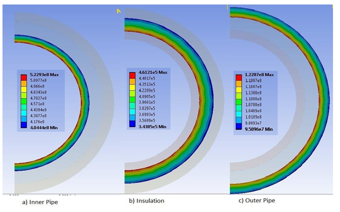
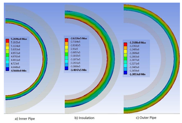
Figure 8 shows the hoop stress recorded on each component of the PIP system. As is expected, the maximum hoop stress is located on the inner surface for the inner pipe and insulation whilst it is on the outer surface for the outer pipe. The inner pipe has a maximum internal hoop stress of 526.96MPa. The hoop stress on the insulation layer ranges from -0.348MPa to -0.262MPa and then from -138.53MPa to -121.08MPa on the outer pipe.
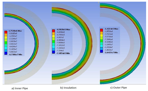
The radial stresses are shown in Figure 9. The results show that the inner pipe exhibits the highest radial stresses compared to the installation material and the outer pipe. This ranges from -67.306MPa on the inner surface to 1.754MPa on the outer surface. On the other hand, the insulation material shows relatively similar values of radial stresses between the inner and outer surfaces as shown. The radial stress on the inner surface of the insulator is -0.750MPa at the inner radius. While, on the outer surface is computed and found to be -0.658MPa at the outer radius. The outer pipe shows radial stresses to varies from -0.142MPa on the inner surface to - 16.437MPa on the outer surface. This variation is attributed to external load of 14.47MPa applied to the model.
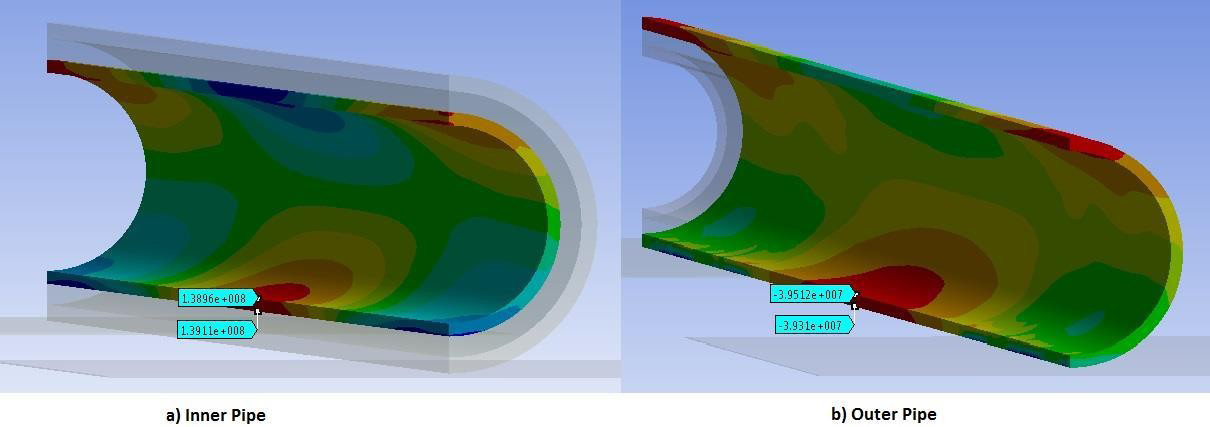
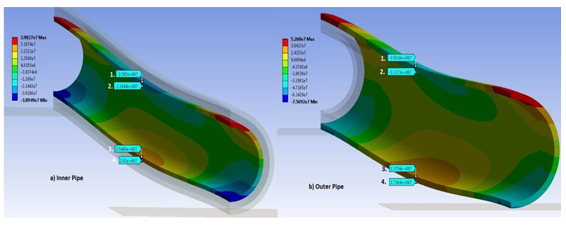
The axial stresses at the points of bending are computed and presented by the data labels in Figure 10. Stresses on the inner and outer surfaces of the inner pipe are 138.96MPa and 139.11MPa respectively. Similarly, for the outer pipe it was computed and found to be -39.512MPa on the inner surface and -39.31MPa at the outer surface.
Effect of Longer Free Span in PIP System
A new model was built with the exact same settings as the 8m PIP in free span with pressure loading however the length of the pipe was increased from 8m to 30m. The seabed sections remained unchanged meaning the section of the PIP system in free span was 26m.
Figure 11 shows the axial stress. As it can be seen, Figure 11a) shows the inner pipe which has a maximum axial stress of -19.373MPa and a minimum of -169.64MPa. The axial stress on the insulation layer ranges from - 0.506MPa (the maximum value) to -0.629MPa. The outer pipe is subjected to a maximum axial stress of 107.47MPa and a minimum of -113.91MPa.
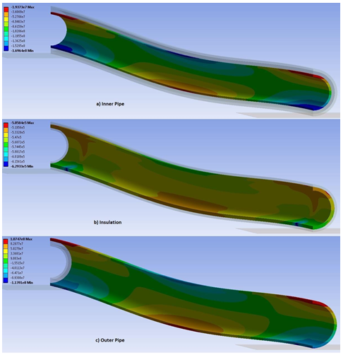
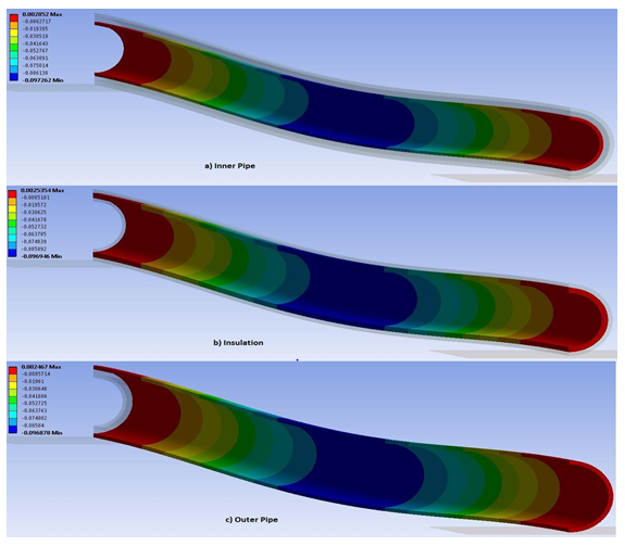
The model was solved to determine the von Mises, hoop, radial and the Y axis deformation for each layer of the PIP system. The Y axis deformation for each layer is shown in Figure 12. The maximum deflections are all located at the midpoint of the model. The inner pipe deflects downwards 0.0973m, the insulation layer 0.0969m and the outer pipe also 0.0969m.
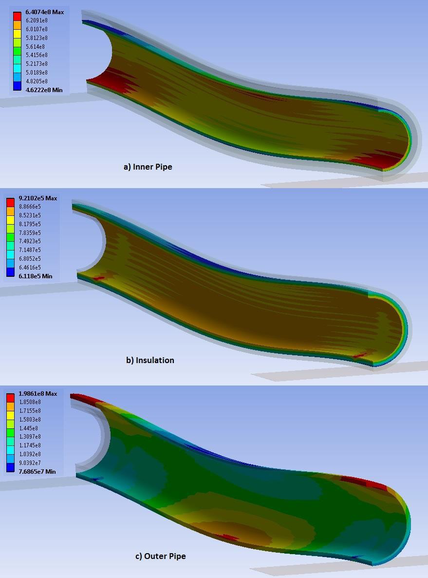
The calculated von Mises stress for the inner pipe ranges from the maximum of 640.74MPa to a minimum of 463.22MPa. On the other hand, the insulation material shows a very low values of von Mises stress with maximum of 0.921MPa and a minimum of 0.612MPa. The outer pipe, however, exhibit 198.61MPa and 76.87MPa foe the maximum and the minimum respectively. These results are presented on Figure 13.
The hoop stress follows the same pattern along the length therefore only the wall thickness needs to be shown in Figure 14. The inner pipe, as can be seen by a) in the Figure (14) has maximum and minimum values of 525.2MPa and -67.703MPa. The insulation maximum hoop stress is - 0.454MPa and the minimum is -1.364MPa. On the outer pipe the stress ranges from -1.229MPa to -149.86MPa.
s
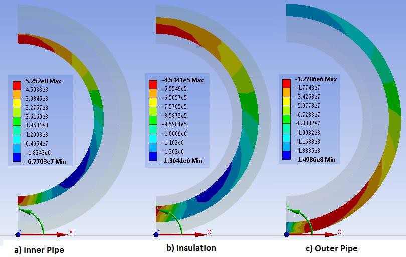
The radial stresses are shown in Figure 15. The inner pipe is subjected to radial stresses ranging from -64.849MPa to 521.05MPa, a much larger range than experienced by the insulation. The maximum radial stress on the insulation is -0.448MPa with a minimum of -1.480MPa. The outer pipe has maximum and minimum values of -0.669MPa and -149.86MPa respectively.
Further analysis on the calculated bending stresses at a point of bending is presented on Figure 16. The results for the locations 1-4 are summarised and compared with theoretical calculations of simply and fixed supported beam in Table 3. The Table clearly shows that the FEA results, for both the inner and outer pipes lies between the simply supported and fixed values. This validates the procedure used to calculate the bending stresses. It also adds weight to the reason given stating that having 50% of a short model constrained the way it may affect the results.
| Inner Pipe Bending Stress (MPa) | Outer Pipe Bending Stress (MPa) | |||||
|---|---|---|---|---|---|---|
| Location | FEA | Simply | Fixed | FEA | Simply | Fixed |
| 1 | -25.85 | -38.88 | -12.96 | -35.02 | -51.86 | -17.29 |
| 2 | -22.84 | -34.41 | -11.47 | -31.17 | -46.29 | -15.43 |
| 3 | 25.49 | 34.41 | 11.47 | 33.75 | 46.29 | 15.43 |
Table 3: Bending stress comparison between theory and FEA for 30m free span length of the PIP system.
Table 4 compares the deflection of each layer of the PIP system when subjected to the different loading conditions. The deflection is in millimetres and indicate a downwards displacement. From the results it can be seen that the deflection of each layer increases as more loads are applied to the model, this indicates each loading condition adds to the amount of bending the system is subjected to.
| Deflection (mm) | ||||
|---|---|---|---|---|
| Model | Inner Pipe | Insulation | Outer Pipe | |
| PIP in Free Span | 8m Gravity | 0.376 | 0.375 | 0.375 |
| 8m Pressure | 1.114 | 0.894 | 0.895 | |
| 8m Pressure & Temperature | 1.368 | 1.151 | 0.989 | |
| 30m Pressure & Temperature | 97.262 | 96.946 | 96.878 |
Table 4: Comparison between the models for deflection.
The 30m single pipe in free span (with pressure and temperature) deflected 205.1mm, more than double the corresponding PIP model. The three layers, particularly the steel pipes combine to significantly increase the stiffness of the system which results in less bending. This agrees with the work of Harrison and Helle [32] which combined the stiffness of both pipes whilst creating an equivalent pipe-in- pipe model. This proves one of the advantages of PIP systems in that the design provides a greater amount of protection to the inner pipe carrying HPHT fluids.
Conclusion
Stress analysis and the phenomenon of pipeline free spans is modelled, and simulation results presented together with risks associated with free spanning pipelines. Finite element models were analysed for both single pipe and pipe- in-pipe (PIP) configurations, these models were situated on a 4m span and 26m span. The free span models utilised gravity loading in addition to the pressure and thermal loadings and included both a single pipe and PIP model with only gravity loading.
The technology and complexity of a PIP system was presented along with advantages and disadvantages of employing the PIP system for a subsea tieback. The various stresses that included von Mises, axial, hoop, and radial of all the components of the computed and presented. In addition, the effect of point bending, and the corresponding deflection of the PIP are examined and comparison made a conventional single pipeline. Various theoretical calculation was used to verify the FEA results of the PIP system. Relevant piping codes and standards were highlighted to show the importance of safe operations and consistent designs to the oil and gas industry.
References
-
Bai Y, Bai Q (2005) Subsea pipelines and risers_._ 1st(Edn.), Elsevier, pp: 809-812.
-
Dos Reis E, Sphaier L, Nunes L, Alves LSDB (2018) Dynamic response of free span pipelines via linear and nonlinear stability analyses. Ocean Engineering 163: 533-543.
-
Zakeri A (2009) Submarine debris flow impact on suspended (free-span) pipelines: Normal and longitudinal drag forces. Ocean Engineering 36(6-7): 489-499.
-
Barrette P (2011) Offshore pipeline protection against seabed gouging by ice: An overview. Cold Regions Science and Technology 69(1): 3-20.
-
Saha D, Hawlader B, Dutta S, Dhar A (2019) Effects of Seabed Shear Strength and Gap Between Pipeline and Seabed on Drag Force on Suspended Pipelines Caused by Submarine Debris Flow. The 29th International Ocean and Polar Engineering Conference, Honolulu, Hawaii, USA.
-
Silva L, Teixeira A, Soares CG (2019) A methodology to quantify the risk of subsea pipeline systems at the oilfield development selection phase. Ocean Engineering 179: 213-225.
-
Chayeb ARE, Wang DX, Kamal FR, Takieddine O (2019) Advanced Pipeline Crossing Analysis. The 29th International Ocean and Polar Engineering, Honolulu, Hawaii, USA.
-
Berntsen J, Furnes G (2002) Small scale topographic effects on the near seabed flow at Ormen Lange. Technical report no. 171, Department of Applied Mathematics, University of Bergen Bergen, Norway.
-
Nikoo HM, Bi K, Hao H (2018) Effectiveness of using pipe-in-pipe (PIP) concept to reduce vortex-induced vibrations (VIV): Three-dimensional two-way FSI analysis. Ocean Engineering 148: 263-276.
-
Bi K, Hao H (2016) Using pipe-in-pipe systems for subsea pipeline vibration control. Engineering Structures 109: 75-84.
-
Bruton D, White D, Cheuk C, Bolton M, Carr M (2006) Pipe/soil interaction behavior during lateral buckling, including large-amplitude cyclic displacement tests by the safebuck JIP. Offshore Technology Conference, Houston, Texas, USA.
-
Mohammed AI, Oyeneyin B, Bartlett M, Njuguna J (2020) Prediction of casing critical buckling during shale gas hydraulic fracturing. Journal of Petroleum Science and Engineering 185: 106655.
-
Auwalu I, Zahra I, Adamu M, Usman A, Sulaiman A (2015) Effectiveness of Simulations on Well Control during HPHT well drilling, SPE Nigeria Annual International Conference and Exhibition_,_ Society of Petroleum Engineers, Lagos, Nigeria.
-
Fish Safe (2009) Pipelines. Aberdeen, Scotland.
-
Bakhtiary AY, Ghaheri A, Valipour R (2007) Analysis of offshore pipeline allowable free span length. International Journal of Civil Engineering 5(1): 84-91.
-
DNV (2010) Interference between trawl gear and pipelines. Recommended Practice DNV-RP-F111, Det Norske Veritas, Norway.
-
Furnes G, Berntsen J (2003) On the response of a free span pipeline subjected to ocean currents. Ocean Engineering 30(12): 1553-1577.
-
Binazir A, Karampour H, Sadowski AJ, Gilbert BP (2019) Pure bending of pipe-in-pipe systems. Thin-Walled Structures 145: 106381.
-
Wang L, Tang Y, Ma T, Zhong J, Li Z, et al. (2020) Stress concentration analysis of butt welds with variable wall thickness of spanning pipelines caused by additional loads. International Journal of Pressure Vessels and Piping 182: 104075.
-
Shah BC, White CN, Rippon IJ (1988) Design and operational considerations for unsupported offshore pipeline spans. SPE Prod Eng 3(2): 227-237.
-
Veritas DN (2006) Recommended practice DNV- RP-F105: free spanning pipelines. DNV, Oslo.
-
Aspen Aerogels (2012) Subsea Thermal Insulation. Northborough, MA, Aspen Aerogels.
-
Mohammed AI, Oyeneyin B, Atchison B, Njuguna J (2019) Casing structural integrity and failure modes in a range of well types-a review. Journal of Natural Gas Science and Engineering 68: 102898.
-
Prathuru AK, Faisal NH, Jihan S, Steel JA, Njuguna J (2016) Stress analysis at the interface of metal-to-metal adhesively bonded joints subjected to 4-point bending: Finite element method. The Journal of Adhesion 93(11): 855-878.
-
Alary V, Marchais F, Palermo T (2000) Subsea water separation and injection: A solution for hydrates. The Offshore Technology Conference, Houston, Texas.
-
Dixon M (2013) Pipe-in-Pipe: Thermal management for effective flow assurance. Offshore Technology Conference, Houston, Texas, USA.
-
Harrison GE, Kershenbaum NY, Choi HS (1997) Expansion analysis of subsea pipe-in-pipe flow line. The Seventh International Offshore and Polar Engineering Conference, Honolulu, Hawaii, USA.
-
Bokaian A (2004) Thermal expansion of pipe-in-pipe systems. Marine Structures 17(6): 475-500.
-
Joshi S, Prashant A, Deb A, Jain SK (2011) Analysis of buried pipelines subjected to reverse fault motion. Soil Dynamics and Earthquake Engineering 31(7): 930-940.
-
Ghoi HS (1995) Expansion analysis of offshore pipelines close to restraints. The Fifth International Offshore and Polar Engineering Conference, Hague, Netherlands.
-
ANSYS (2014) Solid186. ANSYS Inc.
-
Harrison RI, Helle Y (2007) Understanding the response of pipe-in-pipe deep water riser systems. The seventeenth international offshore and polar engineering conference, Lisbon, Portugal.
- Nigeria’s Vulnerability in the Face of Global Energy Policy
- A Simulation Study of Investigation of Optimum Oil Production Performance by Applying Various Gas Injection Methods in Oil Reservoir
- Characterization of Permo-Triassic Reservoirs through Thermal Maturity Assessment of Westphalian Source Rocks in the Cheshire Basin
- Influence of Microwax on the Rheological and Thermal Behaviour of a Wax Crude Oil
- Real-Time Monitoring and Performance Optimization of Steam Injection in Heavy Oil Reservoirs Using Fiber Optic Sensing and Integrated Predictive Simulation Models
- Rapid On-Site Determination of the Total Petroleum Hydrocarbon Content of Soils by Handheld Fourier Transform Near-Infrared Spectroscopy: Development of a Global, Site- and Scanner- Independent Calibration Model