Mathematical Modification to the Classical Volumetric Method for Estimating Oil Reserves
Using fuzzy logic technique, this work proposes a mathematical adjustment to the classical volumetric method for estimating oil reserves to manage the level of uncertainty associated with oil reserves estimation. This technique introduces a risk factor (α) into the volumetric method equation to account for the uncertainty associated with estimating the parameters that are used in the volumetric method equation. Risk types that may affect oil reserves estimation can be considered using the risk factor (α) in the modified equation. Results showed that the amount of proven oil reserves decreases exponentially as the value of risk factor (α) increases. It also showed that the ratio of the expected proven oil reserves with respect to proven oil reserves (N*/N) goes to zero when the value of risk factor (α) reaches a value of (5). Three cases were proposed to categorize uncertainty in proven oil reserves estimation: high risk estimate, middle risk estimate and risk-free estimate. Results showed that, for the case of high-risk estimate, expected proven oil reserves (N*) was appreciably lower than the proven oil reserves (N) due to the inclusion of risk. Sources of risk may include, but not limited to, lack of expertise of the evaluator, level of integrity of the evaluator, engineering errors during measurement and calculation and governmental laws. Results also showed that the calculated amount of proven oil reserves (N*), for the middle risk estimate case, is much higher than that for high risk estimate case. As for the riskfree estimate case, the calculated proven oil reserves (N*) using the modified formula equals to the proven oil reserves (N) calculated by the classical volumetric formula. This case reflects 100% confidence and reliability in the parameters’ estimation which also places great trust in the evaluator’s integrity and expertise.
Introduction and Background
The quantities of petroleum that are expected to be commercially recoverable from known accumulations for a given interval of time are called reserves. Reserves estimation is the process of evaluating quantitative economical recoverable hydrocarbons in a specific area. The level of uncertainty in reserve estimation mainly depends on the geological and engineering data reliability available at the estimation time, and how this data was interpreted. Uncertainties can be financial, political, and contractual [1, 2, 3].
A general classification was established based on the degree of uncertainty and it consists of two major classes of reserves; proved and unproved [4, 5] as shown in Figure 1.

Proved Reserves are the quantities of hydrocarbons that can be measured with certain reliability to be commercially recoverable, by analyzing geological and engineering data , from a given date forward, from known reservoirs and under current economic conditions, operating methods, and government regulations [6].
Developed producing reserves are producing reserves from existing wells from completion interval(s) open to production. Developed nonproducing reserves are those reserves at minor depths below the producing zones proved already by production either from other wells in the field or by core analysis from the particular zones. Adding additional costs can make these reserves productive. The undeveloped reserves are proved for production by reasonable geological and engineering interpretation of nearby producing reservoirs or proved by other wells, but are not recoverable from present wells within the reasonably predictable future, requiring drilling of additional wells, deepening of present wells, or plugging-back and perforating of zones behind the casing of present wells. Unproved reserves are either probable or possible. Probable means that these reserves are uncommercially recoverable reserves depending on their geological and engineering data analysis. Possible reserves are reserves with less chance of having commercial recoverable hydrocarbon amount than probable reserves [7].
Methods of Reserves Estimation
Volumetric method is the most common method and the scope of this paper. Calculations in this method depends on the volume of the reservoir that can be calculated through maps and petrophysical data of the drilled wells. It is an early-stage method applied after completion. Neglecting the reservoir heterogeneity and including undrained compartments that do not affect the flow but presented in the bulk rock volume of the reservoir or accumulation, result in high estimate value [8].
The amount of initial oil in place can be computed after volume calculations using reservoir characteristics (porosity and water saturation) and fluids properties (formation volume factor) by the following formula ( ) 7758 1 o w V Ø S N B $$ = \frac {7 7 5 8 V _ {o} \O \left(1 - S _ {w}\right)}{R} \tag {1} $$ o Another common method is the material-balance method which needs reliable pressure data and PVT data describing the reservoir’s fluids behavior. A constant pore volume (PV) of a reservoir with the reservoir pressure drop during production is assumed. Pressure is inversely proportional to Volume so; a material balance is used to calculate the fluids volumes of the reservoir to illustrate the expansion for the observed pressure drop. Reliability of this method depends on how accurate is the history of the average reservoir pressure, precise production data, and reservoir fluids PVT data. Sources of Error in the Estimation Process Assumptions can be a source of error sometimes. One of the assumptions in volumetric method is that the volume of the pore space in the reservoir occupied by gas and oil is constant. Another assumption is that the reservoir initially filled with liquid or that a definite quantity of the reservoir contained gas. Calculations based on the lab samples will assume that the oil and gas behavior in the laboratory similar to their reservoir behavior under similar conditions of temperature and pressure [9].
Other than the assumptions, some data are interpolated or extrapolated to approximate some values such as bottom- hole pressures, quantities of oil and gas production, and deviation of gases from the ideal [10].
The highest level of uncertainty is detected in early stages of development of reservoir life, boundary areas or wherever a new technology is being applied [11, 12]. Errors are either geological which are related to mapping surfaces, downdip limits, isopachous maps and attic volumes, or engineering errors related to decline curves of composite field, and neglecting minimum hyperbolic decline rate application [13].
Prior Work
Probabilistic method using computer applications and statistical analysis, where each variable is described using a relative frequency curve by a range of possible values of it. Monte-Carlo or similar method is used to estimate the reserves. Repeating this procedure will assist to create a frequency distribution curve that describes the range of estimates and the probability of achieving particular estimates [14].
Igbokwe and chidozie [15] used MBAL (Multi-Block Algorithm) software to compute the oil originally in place but for further studies they suggested that it may not be accepted as accurate compared to a more robust approach which is building dynamic models that may be considered more reliable option since these models consider the interferences in the reservoir resulting from operational changes occurring in the reservoir (pressures, rates) which in turn affect other PVT parameters, one example is Eclipse. Another work enhancing by adjusting the contrast in hydrocarbon-in place volumes from volumetric estimate through fluid contact points which might have been poorly delineated. Karacaer and Onur [16] presented an analytical uncertainty propagation method which they called (AUPM) to model uncertainties on volumetric reserve estimations. They derived AUP equations (AUPEs) using Taylor-series expansion as a basis around the mean values of the input variables. They conducted comparative studies to prove the AUPM accuracy and compare it to the Monte Carlo method (MCM) accuracy. They have the same level of accuracy but the AUPM is faster than the Monte Carlo simulation. They also presented a variable called uncertainty percentage coefficient to simulate the uncertainty effect of each parameter and correlated parameter pairs to the total uncertainty in volumetric calculations. Another method was proposed by them, which is the uncertainty sorting method (USM) that works for determining pair-wise correlation coefficients for multiple resources to provide an analytical approach that is easy to apply and fast which takes the uncertainty percentage coefficient of individual field parameters as a basis. These proposed analytical models can be used as a quick tool to eliminate the need for Monte Carlo Simulation.
Material and Methods
Calculations of oil and gas volumes by STB is carried out in the volumetric method taking the reservoir rocks and fluids physical properties as a basis. The volumetric method depends on the following parameters in reservoir-volume estimation:
- Reservoir size (height or thickness and area).
- Physical reservoir rock properties like porosity ( Ø ) and water saturation (Swi).
- Physical reservoir fluids properties like formation volume factor (Bo).
After estimating or determining these parameters, initial oil in place (N) can be calculated using the following formula:
( ) 7758 1 wi S Ah N B
ϕ − = (2) o In this paper only oil reserves are considered. The technical limitations associated with using volumetric method include; shortage in accuracy and reliability of reservoir size, reservoir rocks and fluids physical-properties. Other than that, these properties are usually measured under lab conditions, which do not represent real reservoir conditions [17, 18].
A major concern when employing the volumetric method for oil reserves estimation is the uncertainty associated with determining (estimating or measuring) the parameters involved in equation 2 such as reservoir porosity, water saturation, thickness, area and oil formation factor. Most often than not, evaluators tend to overestimate these parameters leading to an exaggerated oil reserves volume [19, 20]. Mathematical Adjustment Equation 2 was proposed using fuzzy logic technique to manage the level of uncertainty associated with oil reserves estimation. This technique introduces a risk factor (α) into equation 2 to account for the uncertainty associated with estimating the parameters that are used in equation 2 as mentioned above. The new modified volumetric equation calculates the adjusted proven oil reserves (N *) as follows:
( ) * 7758 1 Ø S Ah N e B
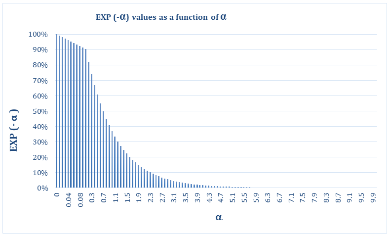
$$ = e ^ {- \alpha} \frac {7 7 5 8 \O \left(1 - S _ {w}\right) A h}{B} \tag {3} $$ w o When the risk factor (α) equals to zero it means there is no risk involved, and that makes the adjusted proven oil reserves (N *) equals to 100% of original estimation of proven oil reserves (N). But, any other value of (α) means that the estimation of proven oil reserves is at risk; and it may be less than 100% of original estimation of proven oil reserves (N). Deviation from 100% (N), naturally, depends on the amount of risk involved, expressed by (α), as shown in Figure 2.
New Formula
Considering the effect of each risk type, as mentioned above (from 1-5), on the value of (α ) may differ, so, a new formula is proposed to take both risk factor and risk weight into account for each risk type, as follows:
n $$ \alpha = \sum_ {i} ^ {n} \gamma w \tag {4} $$
Three risk types will be focused on purposely in the proposed work which are porosity, water saturation and reservoir height. These three risk parameters were chosen because they are relevant to all reservoirs. Furthermore, sufficient published data is available to evaluate these risk types. Other types of risk associated with other parameters will be included in the future. Each risk type has its own risk weight (%) as shown in Table 1.
| Risk Type | Risk Weight (w) % |
|---|---|
| Porosity | 50% |
| Water saturation | 25% |
| Reservoir Height | 25% |
Table 1: Risk sources and their contributed risk weights (w)%.
Porosity has more risk weight than the other two risk types which reflects its importance in proven oil reserves estimation; while assigning equal risk weights (%) for water saturation and reservoir height parameters.
Further procedure in the proposed methodology was to qualitatively classify and determine a risk factor (γ ) for each risk type as shown in Table 2.
| Reliable Estimates | 50% Estimate Reliability | Non-Reliable Estimates |
|---|---|---|
| 0 | 0.5 | 1 |
Table 2: Assigned risk factor (α) for risk categories.
Discussion & Analysis
Three hypothetical cases, shown in Table 3, with three different scenarios are discussed to estimate oil reserves, using equation 2, and observe how both risk-impact weight %(w) and risk-impact factor (γ ) could be assigned unprejudiced.
| Reservoir | Area (ft2) | Thickness (ft) | Porosity φ | Water saturation (S ) wi | Formation volume factor (B ) o | Reserves (STB) Equation (3.1) |
|---|---|---|---|---|---|---|
| 1 | 26,900 | 65.6 | 0.15 | 0.7 | 1.02 | 6.04E+08 |
| 2 | 32,292 | 98.4 | 0.2 | 0.72 | 1.15 | 1.20E+09 |
| 3 | 37.674 | 131.2 | 0.25 | 0.75 | 1.18 | 2.03E+09 |
Table 3: Hypothetical cases for three oil fields.
The three scenarios are: high risk estimate, middle risk estimate and risk-free estimate. The discussion will be purposely limited to (3) risk types: porosity, water saturation and reservoir height. Moreover, the risk weights (%) shown in Table 1 will be used.
High Risk Estimate Calculations
In this case, a risk factor (α) of (1) is assigned to all risk types. Risk weights shown in Table 1 will be used. The risk factor (α) is computed using Equation 4 and the expected proven oil reserves (N*) using Equation 3 for the three reservoirs as shown in Table 4 and Figure 3. The calculated risk factor (α) equaled 1 and the subsequent e-a was calculated to be 0.368.
| Reservoir | Reserves Estimate (N) (STB) | EXP (α ) | Reserves Estimate (N*) (STB) |
|---|---|---|---|
| 1 | 6.04E+08 | 0.368 | 2.21E+08 |
| 2 | 1.20E+09 | 0.368 | 4.40E+08 |
| 3 | 2.03E+09 | 0.368 | 7.50E+08 |
Table 4: Reserves estimate (N) versus reserves estimate (N*) for reservoirs 1, 2 & 3 for high risk estimate.
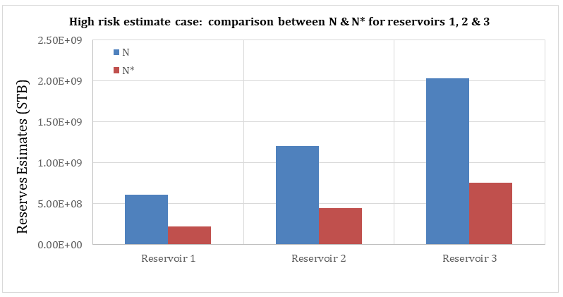
It can be seen from Table 4 and Figure 3 that the expected proven oil reserves (N*) calculated by Equation 3 is appreciably lower than the proven oil reserves (N) calculated by Equation 2 due to the inclusion of risk. This risk is driven by the uncertainty in gathering the parameters used in Equation 2. The sources of uncertainty may include, but not limited to, lack of expertise of the evaluator, level of integrity of the evaluator, engineering errors during measurement and calculation and governmental laws. The calculated (N*) should be used as a benchmark for proven oil reserves to avoid technical and economic problems especially those related to engineering facility planning and budget requirements. The difference between (N) and (N*) could be reduced by following standard measurements and testing procedures such as those suggested by American Petroleum Institute (API). In addition, selecting an evaluator with integrity and expertise will definitely lessen the difference between (N) and (N*). Moreover, avoiding design and calculations mistakes help in alleviating errors when calculating (N).
Middle Risk Estimate Calculations
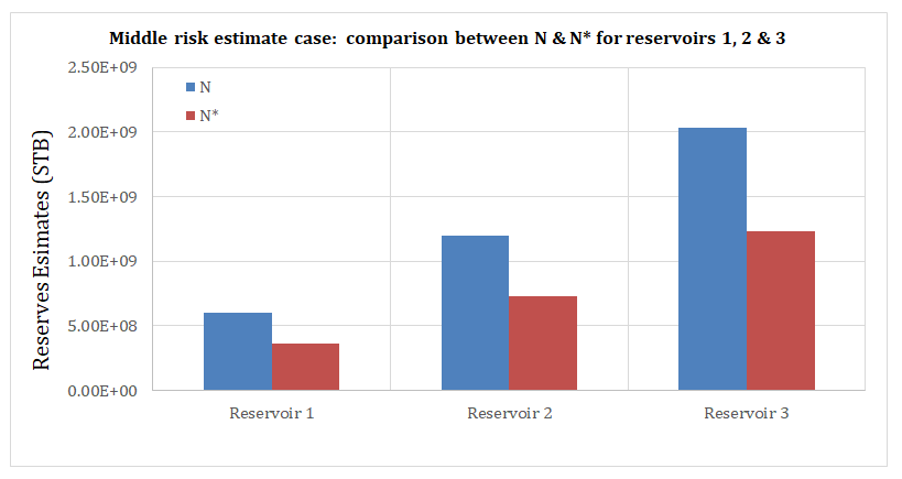
In this case, a risk factor (α) of (0.5) is assigned to all risk types under consideration; porosity, water saturation and reservoir thickness. Furthermore, a risk weight of 50%, 25% and 25% is assigned to porosity, water saturation and reservoir thickness respectively.
The calculated risk factor (α) equaled 0.5 and the subsequent e-a was calculated to be 0.6065.
It can be seen from Table 5 and Figure 4 that the amount of proven oil reserves (N*) calculated by Equation 3 for the middle risk estimate case is much higher than that for high risk estimate case. Using a risk factor (α) of (0.5) has increased the amount of proven oil reserves (N*). This reflects more confidence and reliability of the parameters’ estimation than the case of high-risk estimate where the risk factor (α) was set to be (1). One can set the risk factor (α) to be less than 1 if the parameters’ estimation process carries less risk and have been conducted by professionals who have expertise in the field, and according to professional measurement and testing standards. Values of the risk factor (α) may vary between (1) for extreme risk to (0) for no risk situations.
| Reservoir | Reserves Estimate (N) (STB) | EXP (-α ) | Reserves Estimate (N*) (STB) |
|---|---|---|---|
| 1 | 6.04E+08 | 0.6065 | 3.66E+08 |
| 2 | 1.20E+09 | 0.6065 | 7.30E+08 |
| 3 | 2.03E+09 | 0.6065 | 1.23E+09 |
Table 5: Reserves estimate (N) versus reserves estimate (N*) for reservoirs 1, 2 & 3 for middle risk estimate.
Risk-Free Estimate Calculations
In this case, a risk factor (γ ) of (0) is assigned to all risk types under consideration; porosity, water saturation and reservoir thickness. Furthermore, a risk weight of 50%, 25% and 25% is assigned to porosity, water saturation and reservoir thickness respectively. The calculated risk factor (α) equaled 0 and the subsequent e-a was calculated to be 1.
| Reservoir | Reserves Estimate (N) (STB) | EXP (-α ) | Reserves Estimate (N*) (STB) |
|---|---|---|---|
| 1 | 6.04E+08 | 1 | 6.04E+08 |
| 2 | 1.20E+09 | 1 | 1.20E+09 |
| 3 | 2.03E+09 | 1 | 2.03E+09 |
Table 6: Reserves estimate (N) versus reserves estimate (N*) for reservoirs 1, 2 & 3 for risk-free estimate.
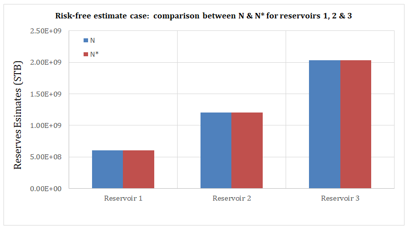
This case reflects 100% confidence and reliability in the parameters’ estimation which also places great trust in the evaluator’s integrity and expertise. For this reason, the proven oil reserves (N*) calculated by Equation 3 equals the proven oil reserves (N) calculated by Equation 2 as shown in Figure 5 and Table 6. In other words, the risk and associated uncertainty has been eliminated due to the accuracy and reliability of the perimeters’ estimation process. To achieve this state, strict procedures must be followed when estimating porosity, water saturation and reservoir thickness parameters. Measurements and testing must strictly follow standard API procedures and acceptable international methods.
Sensitivity Analysis
To have a better picture of the effect of risk factor (α) on the overall proven reserve’s estimation, the following sensitivity analysis has been conducted by changing the risk factor (α) values from (0) to (1) and recalculate the expected proven oil reserves (N*) following the same method used above. Figure 6 shows proven oil reserves (N*) as a function of risk factor (α) for reservoirs 1, 2 and 3.
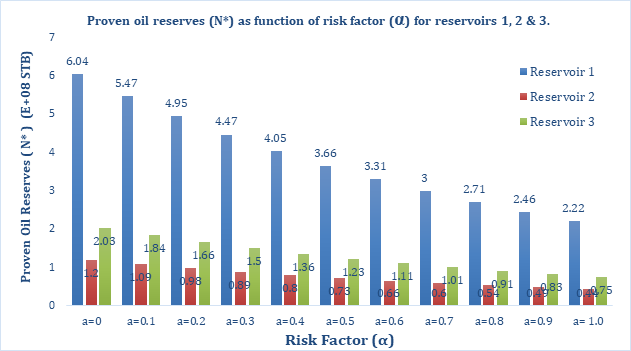
It can be seen from Figure 6 that the amount of proven oil reserves (N*) decreased as the value of risk factor (α) increased from (0) to (1). This is expected since, according to the model, the amount of risk and uncertainty increases as the risk factor (α) increases beyond a value of (0) which represents a risk-free point. It is possible to have a risk factor value (α) greater than (1). Risk factor (α) values greater than (1) reflect more uncertainty associated with the parameters’ estimation process. Figure 7 shows the expected proven oil reserves (N*) with respect to proven oil reserves (N) as a function of risk factor (α).
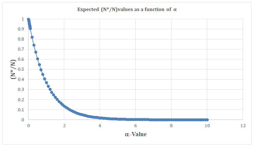
Figure 7 shows that the amount of proven oil reserves decreases exponentially as the value of risk factor (α) increases. It can also be seen that the ratio of (N*/N) goes to zero when the value of risk factor (α) reaches around (5). This means that the higher the amount of uncertainty in parameters’ estimation, the lower the amount of expected proven oil reserves (N*). Some countries deliberately fake out data related to reservoir parameters in order to obtain high values for their proven oil reserves. Declaring high risk estimate values for economic purposes is a thing that most oil-producing countries do. Serious economic consequences may be result from this unethical, irresponsible, and untransparent practice not only on the country itself but also on the whole world. Wrong or overstated reserves figures may give a false sense of security regarding global oil supply and this will result in huge efforts of development and deployment of other energy resources [21].
Conclusion and Future work
Referring to the newly modified formula (Equation 3), proven oil reserves estimates could drop sharply if one considers uncertainties and risks associated with the parameters’ estimation process. Such parameters include porosity, water saturation, reservoir area, height and oil formation factor.
The use of (α) factor in the modified equation make it easier to us to study all types of risks that could affect proven oil reserves estimation. This becomes possible when equation 4 is used, where (α) factor is evaluated from risk factor (γ ) and risk weight %(w) for each risk type. Assigning numerical values to (γ ) and (w) factors, for each risk type, to reflect their respective risk levels presents a major challenge and requires expert opinion. Therefore, an expert opinion is important when evaluating (γ ) and (w) factors.
This analysis showed that the amount of proven oil reserves decreases exponentially as the value of risk factor (α) increases. It also showed that the ratio of adjusted reserve estimates to reserve estimates (N*/N) goes to zero when the value of risk factor (α) reaches a value of (5). Eliminating uncertainties and risks associated with proven oil reserves estimation requires high level of accuracy when estimating all parameters used in Equation 2. Accuracy in parameters’ estimation can be greatly improved by following strict procedures when estimating porosity, water saturation, reservoir area and thickness and oil formation factor parameters. Measurements and testing must strictly follow standard API procedures and acceptable international methods. In the future, the types of risks affecting proven oil reserves will be expanded and incorporated into equations 3 and 4 for a better vision of oil and gas sustainability for OPEC countries. Including reservoir area and oil formation factor (Bo) in assessing the uncertainty associated with estimated proven oil reserves will definitely sharpen the understanding of the risks associated with the estimates. Moreover, the risk weight (w%) needs to be refined and incorporated into a sensitivity study so the impact of each factor on the overall proven oil reserves estimates can be seen.
Nomenclature
| (N) | Initial oil in place, STB [stock-tank m3] |
|---|---|
| 7758 | A constant number of barrels per acre-foot |
| ( Ø ) | Reservoir porosity |
| (S ) wi | Reservoir water saturation |
| (A) | Reservoir area (acre) |
| (h) | Reservoir thickness (ft) |
| (B ) o | Formation volume factor, RB/STB [res m3/stock- tank m3] |
| (α ) | Risk factor that accounts for the uncertainty associated with parameters estimations |
| (γ ) | Risk factor for each risk type |
| (w) | Risk weight % for each risk type |
Data Availability Statement
Some or all data, models, or code that support the findings of this study are available from the corresponding author upon reasonable request.
Compliance with Ethical Standards
The authors declare that there was no funding, grants, or other support was received for conducting this study. Moreover, the authors have no relevant financial or non- financial interests to disclose.
References
-
Alhamran M, Loganathan N, Sethi N, Golam Hassan AA (2022) Effects of political stability, oil prices and financial uncertainty on real economic growth of Gulf cooperation council countries. Transnational Corporations Review, pp: 1-14.
-
Martinez AR, McMichael CL (1999) Petroleum reserves: New definitions by the Society of Petroleum Engineers and the World Petroleum Congress. Journal of Petroleum Geology 22(2): 133-140.
-
Wang KH, Xiong DP, Mirza, N, Shao XF, Yue XG (2021) Does geopolitical risk uncertainty strengthen or depress cash holdings of oil enterprises? Evidence from China. Pacific- Basin Finance Journal 66: 101516.
-
AL-Bazali T, Al-Zuhair M (2022) The use of fuzzy logic to assess sustainability of oil and gas resources (R/P): technical, economic and political perspectives. International Journal of Energy Economics and Policy 12(2): 449-458.
-
Demirmen F (2007) Reserves estimation: The Challenge for the Industry. Journal of Petroleum Technology 59(5): 80-89.
-
Poroskun VI, Khitrov AM, Zaborin OV, Zykin MY, Heiberg S, et al. (2004) Reserves/resource classification schemes used in Russia and Western countries: A review and comparison. Journal of Petroleum Geology 27(1): 85-94.
-
Eggleston WS (1962) What are petroleum reserves? J Pet Technol 14(7): 719-726.
-
Sylvester O, Bibobra I (2019) Volumetric Reserves Estimation: Fundamentals and Applications. Springer International Publishing, Germany.
-
Katz DL (1936) A method of estimating oil and gas reserves. Trans 118(01): 18-32.
-
Qun LEI, Dingwei WENG, Jianhui LUO, Zhang J, Yiliang LI, et al. (2019) Achievements and future work of oil and gas production engineering of CNPC. Petroleum Exploration and Development 46(1): 145-152.
-
Rui Z, Lu J, Zhang Z, Guo R, Ling K, et al. (2017) A quantitative oil and gas reservoir evaluation system for development. Journal of Natural Gas Science and Engineering 42: 31-39.
-
Desorcy GJ, Warne GA, Ashton BR, Campbell GR, Collyer DR, et al. (1993) Definitions and guidelines for classification of oil and gas reserves. Journal of Canadian Petroleum Technology 32(5).
-
Harrell DR, Hodgin JE, Wagenhofer T (2004) Oil and gas reserves estimates: Recurring mistakes and errors. the SPE Annual Technical Conference and Exhibition, Houston, Texas.
-
Yadav A, Omara E, El-Hawari A, Malkov A, Bisso Bi Mba EM (2018) Deterministic or Probabilistic Approach for Mature Oilfield Development: Isn’t it all about Decision Making? SPE Russian Petroleum Technology Conference. Moscow, Russia.
-
Igbokwe C (2011) Comparative analysis of reserve estimation using volumetric method and MBAL on niger delta oil fields.
-
Karacaer C, Onur M (2012) Analytical Probabilistic Reserve estimation by volumetric method and aggregation of resources. The SPE Hydrocarbon Economics and Evaluation Symposium, Calgary, Alberta, Canada.
-
Ayoub MA, Elhadi A, Fatherlhman D, Saleh MO, Alakbari FS, et al. (2022) A new correlation for accurate prediction of oil formation volume factor at the bubble point pressure using Group Method of Data Handling approach. Journal of Petroleum Science and Engineering 208: 109410.
-
Al-Bazali TM, Zhang J, Chenevert ME, Sharma MM (2007) Capillary entry pressure of oil-based Muds in shales: The key to the success of oil-based Muds. Energy Sources, Part A: Recovery, Utilization, and Environmental Effects 30(4): 297-308.
-
Rahimov FV, Eminov AS, Huseynov RM (2017) Risk and uncertainty assessment while estimation of reserves. The SPE Annual Caspian Technical Conference and Exhibition, Baku, Azerbaijan.
-
Didar BR, Akkutlu IY (2013) Pore-size dependence of fluid phase behavior and properties in organic-rich shale reservoirs. SPE international symposium on oilfield chemistry. The Woodlands, Texas.
-
Esen V, Oral B (2016) Natural gas reserve/production ratio in Russia, Iran, Qatar and Turkmenistan: A political and economic perspective. Energy Policy 93: 101-109.
- Nigeria’s Vulnerability in the Face of Global Energy Policy
- A Simulation Study of Investigation of Optimum Oil Production Performance by Applying Various Gas Injection Methods in Oil Reservoir
- Characterization of Permo-Triassic Reservoirs through Thermal Maturity Assessment of Westphalian Source Rocks in the Cheshire Basin
- Influence of Microwax on the Rheological and Thermal Behaviour of a Wax Crude Oil
- Real-Time Monitoring and Performance Optimization of Steam Injection in Heavy Oil Reservoirs Using Fiber Optic Sensing and Integrated Predictive Simulation Models
- Rapid On-Site Determination of the Total Petroleum Hydrocarbon Content of Soils by Handheld Fourier Transform Near-Infrared Spectroscopy: Development of a Global, Site- and Scanner- Independent Calibration Model