Prediction of Vapor Liquid Equilibrium of Binary CO2-Contained
Mixtures for Carbon Capture and Sequestration using Artificial
Intelligence

Rostami S; Boukadi F and Hosseini M

doi:10.23880/ppej-16000365

Petroleum & Petrochemical Engineering Journal Research Article 18 min read

Prediction of Vapor Liquid Equilibrium of Binary CO2-Contained Mixtures for Carbon Capture and Sequestration using Artificial Intelligence

Rostami S^*, Boukadi F and Hosseini M

^* Corresponding author

ISSN: 2578-4846 10.23880/ppej-16000365 Received: October 24, 2023 Published: November 20, 2023

— views

49 references

2 figures

5 tables

PDF

Keywords

Carbon Capture and Sequestration Vapor Liquid Equilibrium Machine Learning Thermodynamic Carbon Dioxide Peng Robinson

Abstract

This research provides a comprehensive prediction using machine learning to predict vapor-liquid-equilibrium for CO2- contained binary mixtures for carbon capture and sequestration projects. One of the best practices to lower the CO2 emissions in the atmosphere is Carbon Capture and Sequestration including capturing carbon dioxide from atmosphere and injecting it into the underground geological formations. One of the key elements in a successful project is to accurately model the phase equilibria which provides us on how the fluid or mixtures of the injected fluids will behave in certain pressures and temperatures underground. In this regard, different machine learning models have been implemented for the prediction. The data set consists experimental results of five different binary mixtures with CO2 presents in all of them. Then the results were compared to each other and the one with the highest accuracy was selected for each mixture. Peng Robinson equation of state was also used and compared with machine learning results. Finally, both machine learning and thermodynamic models were compared to experimental results to determine the accuracy. It was found out that thermodynamic model was unable to predict results for many data points while machine learning could predict results for most of the data points. Also, the accuracy of machine learning models was greatly better than thermodynamic model. In this research, a large data set including 748 data points is used on which machine learning models can be trained more accurate. Also, as a single machine learning model cannot predict accurate results for all mixtures, several models have been run on each mixture, and the one with the highest accuracy was selected for each CO2-contained binary mixture which to our knowledge, has been never implemented.

Introduction

Carbon capture and sequestration (CCS) is an efficient method for reducing Carbon Dioxide (CO2) emissions into the atmosphere. CO2 emissions account for a great portion of global warming, and CCS provides a viable strategy for reducing this massive environmental crisis [1, 2, 3]. During every CO2 capture and sequestration project, determination of vapor liquid equilibrium (VLE) which is a state in which a liquid mixture and its vapor coexist in thermodynamic and chemical equilibrium is very challenging and important. VLE is also vital for many applications in chemical engineering, such as distillation, extraction, and absorption. VLE can be used to determine the optimal operating conditions and design parameters for these processes. One of the main factors that affect VLE is the composition of the liquid and vapor phases. The composition of each phase depends on the temperature, pressure, and the nature of the components in the mixture. VLE is important in carbon sequestration because it affects the thermophysical properties of the fluid mixture involved in the capture, transport, and storage of carbon dioxide. For example, VLE determines the solubility of CO2 in water or other solvents, the density and viscosity of the fluid, the energy consumption of the process, and the safety and environmental risks of CO2 leakage. Another challenge associated with carbon sequestration is to model VLE of CO2 and other substances in porous rock formations, where CO2 can be injected and stored. The common-used method for predicting VLE is Thermodynamic models. However, traditional simulators for VLE are computationally expensive and time-consuming, and may not be accurate enough for complex systems. Also, thermodynamic models usually fail in high pressure and temperature which always present during CO2 sequestration projects. To overcome this, artificial intelligence (AI) by using machine learning techniques, such as artificial neural networks (ANNs) can be helpful. AI can also handle complex systems that involve multiple components or phases, which may not be feasible with conventional methods. Vaferi B, et al. [4] used AI to predict VLE for carbon dioxide and refrigerant. Gokulakannan S [5] used AI based model for VLE of CO2 and amines. Aminian A, et al. [6] implemented AI during supercritical conditions for mixtures of CO2 and fatty oils. Also, implementation of machine learning for VLE can be found in Yan Y, et al. [7, 8, 9, 10, 11, 12]. Additionally, Mohanty S [13] used Artificial Neural Network (ANN) for VLE of binary systems. Mesbah M, et al. [14] used LSSVM to predict VLE of CO2 cyclic compounds. Azari A, et al. [15] implemented AI to predict VLE for CO2 binary refrigerant mixtures. Bahmaninia H, et al. [16] used deep learning to predict equilibrium solubility of CO2 in alcohols, and Mehtab V, et al. [17] used machine learning to predict CO2 capture in physical solvents. Also, Liu H, et al. [18] used machine learning to correlate CO2 solubility in tertiary amines. Here, a range of ML models have been used to predict VLE of binary CO2-contained mixtures. In this study, experimental results Hwu WH, et al. [19, 20, 21, 22, 23, 24, 25, 26, 27, 28, 29, 30, 31, 32, 33, 34, 35, 36, 37, 38, 39, 40, 41, 42, 43, 44, 45, 46] collected from literature were used to compare the accuracy of our results. Peng Robinson equation of state is used to calculate thermodynamic data for the corresponding experimental data points. Results showed that the ML models have more accuracy than the thermodynamic models even in high pressures and temperatures which are common during CO2 sequestration operations. Also, the run time is extremely reduced comparing AI to thermodynamic. 748 data points were used during this study. The data base consists of 4 different mixtures including some of the most common components present during carbon capture and sequestration processes including CH4, O2, N2, and H2S. Experimental results comparing the mole fraction of liquid (xi) and mole fraction of vapor (yi) phase when the binary mixture is in equilibrium for all the data points were collected from literature [19, 20, 21, 22, 23, 24, 25, 26, 27, 28, 29, 30, 31, 32, 33, 34, 35, 36, 37, 38, 39, 40, 41, 42, 43, 44, 45, 46]. Then, thermodynamic models were used to predict xi and yi. Finally, 4 Machine Learning (ML) models were used to predict xi and yi. Models have been trained on 70 percent of the data set and tested on the remaining 30 percent. Then, the model with most accuracy for each mixture was selected. We observed that the machine learning models outperform thermodynamic models by 50% in terms of Root Mean Squared Error (RMSE).

Machine Learning Models

Four ML models were used for modeling the VLE, including Decision Trees (DT), Random Forest (RF), Extra Trees (ET), and Lasso Regression (LR).

Decision Trees

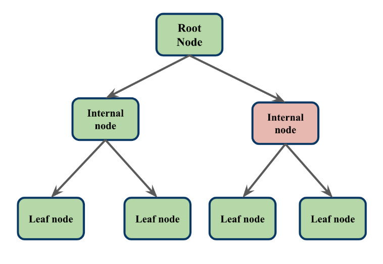
DTs are a non-parametric supervised learning methods used for classification and regression by creating a model that predicts the value of a target variable by learning simple decision rules inferred from the data features. A tree can be seen as a piecewise constant approximation. decision trees are consisted of root node, branches, internal nodes and leaf nodes [47]. Figure 1 shows a decision tree structure. In each step the decision tree decides how to split the data using Entropy and information gain as below:

() () () 2 log c C Entropy S p c p c =−∑ ò (1) Where S represents the data set that entropy is calculated, c represents classes in set S, p(c) represents the proportion of data points that belong to class c to the number of total data points in set, S, and C represents the class which is a subset of all classes. Also, S InformationGain S a Entropy S Entropy S S = − ∑ ò ( ) () () () , v v v vcalues a (2) In equation 2, a represents a specific attribute or class label, Entropy(S) is the entropy of dataset, S, |Sv|/ |S| represents the proportion of the values in Sv to the number of values in dataset, S, and Entropy(Sv) is the entropy of dataset, Sv.

Random Forest

The random forest model is a machine learning ensemble model that combines several decision tree models and makes decisions using the average decision tree results. In this model, each tree consumes a bootstrap sample of the original data. Like decision trees, the model splits the data using information-gain of the feature. Equation 3 predicts the results of random forest regressor with N trees:

() 1/ i y NSum y = (3)

Where yi is the prediction of the i-th tree. The equation for the prediction of a single decision tree is:

y = f(x) (4) where f(x) is a piecewise constant function that assigns a value to each leaf node of the tree, and x is the input feature vector.

Extra Trees Model

Extra Trees regression like random forest is an ensemble model that uses several decision trees. Extra trees use the best split among all features of the data which makes it more robust in the presence of noise in the data over decision tree and random forest model. A disadvantage of the ET model is more randomness in the model by using the best split over features at each step. The following flowchart shoes the Extra trees. Draw a bootstrap sample Xt,yt from X,y with replacement.

Grow a decision tree on Xt,yt using the following procedure:
For each node,randomly select F features without replacement.
For each feature,randomly select a split point among all possible values.
Choose the feature and the split point that minimize the chosen criterion(squared error,absolute error,etc.) among the F candidates.
Split the node into two child nodes using the chosen feature and split point.
Repeat until the maximum depth is reached or the minimum number of samples at each node is satisfied. Where, ( ) ∝ 1 t ˆ 1/ * y T t y T sum = = (6) where ∝ ty is the prediction of the tth tree for x.

Lasso Regression (LR) is a type of linear regression that performs both variable selection and regularization by adding a penalty term to the ordinary least squares (OLS) objective function. The penalty term is the sum of the absolute values of the regression coefficients, multiplied by a tuning parameter λ. The LR objective function can be written as:

0 1 1 2 2 Y X X pXp β β β β ε = + + ++ + (7) Where,

: Y Theresponsevariable

: Xj The jth predictor variable : , j Theaverageeffect onY of aoneunitincreasein Xj holding all other predictors fixed β : Theerrorterm ε The LR method removes the effect of the less important predictors toward zero by reducing their coefficients which reduces the model complexity.

Thermodynamic Model

To generate thermodynamic results, the Peng Robinson (PR) equation of state (EoS) was used through “pypi” in PYTHON. The following form of PR EoS has been implemented (Equation 8 & 9) [48].

() ( ) ( ) a T RT P v b v v b b v b = − − + + − (8)

i i i i i 

1 1

8.314472 . .

− − = R Jol mol K RT b Pc i c i

0.0777960739 = p i p

2 2 2         = + −             ≤ = + −

R T T with a m Pc i Tc i c i

0.457235529 1 1 p i i p p

2

0.491... 0.37464 1.5422 0.26992 if m ω ω ω i i i i  = + − + 2 016666 i ω

2

0.491... 0.379642 1.48503 0.164423 0.

if m ω ω ω i i i i (9)

In “pypi” all critical properties of different mixtures and components are defined, making it efficient to calculate VLE properties.

Results

We trained the models on 70 percent of the data and tested the model on the 30 percent remainder and compared the predictions with the experimental results. Table 3 to Table 6 Show the performance of the models compared to thermodynamics models. ET outperforms other ML

Bootstrap	False
ccp_alpha	0
criterion	squared_error
max_depth	squared_error
max_features	1
max_leaf_nodes
max_samples
min_impurity_decrease	0
min_samples_leaf	1
min_samples_split	2
min_weight_fraction_leaf	0
n_estimators	100
n_jobs	-1
oob_score	FALSE
random_state	4798
verbose	0
warm_start	FALSE

Table 1: Extra-Trees model Hyper-parameters.

Min_sample_leaf	5
Max_depth	15
No_estimators	500
Min_depth	5
Max_features	Auto
bootstrap	True
criterion	mse
Min_impurity_decrease	mse
Random_state	42
Min_sample_split	2

Table 2: Random Forest model Hyper-parameters.

models for N2, O2, H2S reducing the error compared to PR thermodynamic model. However, RF showed better performance in predicting the mole fractions of VLE mixture of CH4 and CO2. Furthermore, we observed the ML models do not function while the data is not sufficient. The codes are publicly available at Hosseini M, et al. [49]. Also, in this paper we used hyper parameter tuning to avoid overfitting the ET and RF models. Table 1-6 Hyperparameters of Et and RF models.

Press (Mpa)	Temp (oF)	X i (exp)	Y i (exp)	X (ther) i	Y (ther) i	X i (ML)	Y i (ML)	Accur. (X- i ML), %	Accur. (Y- i ML), %	Accur. (X- i ML), %	Accur. (Y-ML), % i
7.8	250	0.6	0.395	0.63	0.405	0.618	0.395	95.2	97.43	97.08	100
8.0938	250	0.554	0.442	0.592	0.414	0.554	0.553	93.56	93.3	100	79.92
3.194	270	1	1			1	1	100	100	100	100
4.214	270	0.968	0.838			0.968	0.837			100	99.88
7.02	270	0.887	0.647			0.886	0.647			99.88	100
8.063	270	0.834	0.595			0.839	0.595			99.4	100
0.89166	230	1	1			1	1	100	100	100	100
4.053	230	0.83	0.277	0.833	0.292	0.837	0.277	99.54	94.85	99.16	100
4.8636	230	0.765	0.249	0.773	0.265	0.765	0.241	98.93	93.71	100	96.68
6.190958	230	0.603	0.248	0.631	0.25	0.607	0.248	95.48	99.06	99.34	100
6.934683	230	0.474	0.268			0.47	0.268			99.14	100
6.999531	230	0.457	0.27			0.457	0.275			100	98.18
7.073498	230	0.439	0.275			0.431	0.275			98.14	100
7.140373	230	0.416	0.284			0.416	0.287			100	98.95
2.0265	250	0.99	0.896			0.95	0.475			95.78	11.36
2.362899	250	0.977	0.777			0.971	0.777			99.38	100
4.053	250	0.895	0.509			0.895	0.504			100	99
5.515808	219.26	0.436	0.811	0.596	0.185	0.432	0.811	73.19	0	98.88	100
6.205284	219.26	0.62	0.802	0.596	0.185	0.62	0.802	73.19	0	100	100
4.481594	210.15	0.3604	0.858	0.667	0.141	0.927	0.959	53.96	0	38.86	89.53
4.826332	210.15	0.455	0.86	0.579	0.139	0.73	0.456	78.62	0	62.33	11.35
5.17107	210.15	0.588	0.861			0.588	0.865			100	99.53
5.343439	210.15	0.648	0.86			0.648	0.861			100	99.97
5.688177	210.15	0.754	0.853			0.754	0.853			100	100
4.826332	203.15	0.73	0.891			0.735	0.891			99.41	100
4.89528	203.15	0.749	0.895			0.741	0.895			98.9	100
4.964227	203.15	0.768	0.896			0.76	0.896			98.9	100
5.033175	203.15	0.787	0.897			0.781	0.897			99.11	100
5.102122	203.15	0.805	0.897			0.805	0.895			100	99.7
5.240018	203.15	0.838	0.896			0.838	0.897			100	99.96
5.308965	203.15	0.856	0.893			0.858	0.891			100	99.74
5.336544	203.15	0.878	0.878			0.879	0.878			99.93	100
4.412646	193.15	0.913	0.955			0.913	0.95			100	99.43
4.7367	193.15	0.973	0.973			0.971	0.973			99.73	100
3.378432	183.15	0.939	0.978			0.939	0.977			100	99.84
3.44738	183.15	0.955	0.984			0.955	0.985			100	99.91
3.640433	183.15	1	1			1	1	100	100	100	100
2.482114	173.15	0.956	0.99			0.956	0.9907			100	100
2.516587	173.15	0.968	0.993			0.968	0.991			100	99.76
2.551061	173.15	0.98	0.995			0.98	0.997			100	99.89
1.172109	153.15	0.994	0.999			0.998	0.999			99.66	100
1.175557	153.15	0.997	0.999			0.997	0.992			100	99.24
1.17928	153.15	1	1			1	1	100	100	100	100

Table 3: The predicted xi and yi when the binary mixture is in equilibrium for H2S using thermodynamic and ML model for the five

Press (Mpa)	Tem, oF	X (exp) i	Y i (exp)	X (ther) i	Y (ther) i	X (ML) i	Y (ML) i	Accur. (X- i ML), %	Accur. (Y- i ML), %	Accur. (X-ML), i %	Accur. (Y- i ML), %
6.7764	293.08	0.028	0.082			0.026	0.082			92.83	99.99
6.3196	293.08	0.016	0.052			0.015	0.052			94.77	99.99
7.9718	293.08	0.063	0.136			0.063	0.138			99.99	98.26
8.7359	293.08	0.096	0.145			0.096	0.143			99.99	98.11
8.8928	293.08	0.106	0.144			0.106	0.144			99.99	99.99
4.0872	273.09	0.01	0.102			0.01	0.102			98.05	99.99
9.9653	273.09	0.181	0.397			0.185	0.397			97.73	99.99
10.5708	273.09	0.206	0.391			0.206	0.396			99.99	98.73
10.9443	273.09	0.227	0.383			0.226	0.383			99.38	99.99
11.1974	273.09	0.244	0.371			0.244	0.371			99.95	99.99
11.2488	273.09	0.248	0.368			0.247	0.368			99.23	99.99
11.2967	273.09	0.253	0.364			0.252	0.364			99.56	99.99
11.4268	273.09	0.268	0.347			0.268	0.346			99.99	99.56
11.4992	273.09	0.286	0.331			0.286	0.332			99.99	99.84
7.6582	273.09	0.102	0.36			0.103	0.36			99.51	99.99
6.6602	273.09	0.075	0.32			0.075	0.321			99.99	99.71
2.6882	253.12	0.013	0.213			0.012	0.213			89.43	99.99
3.204	253.12	0.025	0.304			0.02	0.308			74.5	98.67
5.208	253.12	0.707	0.489	0.886	0.483	0.707	0.489	79.73	98.72	99.99	99.95
7.3726	253.12	0.127	0.569	0.806	0.405	0.127	0.405	15.82	59.51	99.99	59.28
10.4707	253.12	0.225	0.591	0.674	0.382	0.253	0.383	33.38	45.39	89.01	45.63
11.433	253.12	0.265	0.58	0.624	0.392	0.265	0.58	42.47	52.04	99.99	99.99
12.7827	253.12	0.344	0.535			0.344	0.534			99.99	99.75
1.205	238.11	0	0			0	0			100	100
2.4946	238.11	0.02	0.447			0.021	0.447			97.14	99.99
3.004	238.11	0.308	0.519	0.934	0.462	0.308	0.519	32.96	87.83	100	99.99
3.9717	238.11	0.549	0.602	0.898	0.378	0.549	0.602	61.1	40.99	99.99	99.99
5.9394	238.11	0.1	0.679	0.823	0.299	0.122	0.679	12.2	0	82.37	99.99
8.9349	238.11	0.189	0.715	0.7	0.266	0.189	0.765	27.08	0	99.99	93.51
11.9705	238.11	0.305	0.69	0.7	0.266	0.305	0.69	27.08	0	99.86	99.99
Press (Mpa)	Temp, oF	X i (exp)	Y ⁱ (exp)	X (ther) i	Y (ther) i	X (ML) i	Y i (ML)	Accur. (X-ther), % i	Accur. (Y-ther), % i	Accur. (X-ML), % i	Accur. (Y-ther), % i
5.731	293.1	0	0			0	0			100	100
6.4864	293.1	0.018	0.066			0.018	0.067			99.99	99.1
6.9772	293.1	0.029	0.097			0.028	0.097			93.57	99.97
8.5942	293.1	0.077	0.146			0.076	0.144			97.63	98.36
8.5868	293.1	0.077	0.146			0.077	0.147			100	99.72
4.2667	273.08	0.015	0.137			0.014	0.135			86.42	98.48
4.9547	273.08	0.029	0.214			0.028	0.209			93.92	97.69
7.3395	273.08	0.078	0.355			0.077	0.351			97.92	99
8.1061	273.08	0.097	0.375			0.096	0.371			98.12	98.79
9.0706	273.08	0.119	0.39			0.119	0.387			100	99.39
11.802	273.08	0.253	0.272			0.253	0.271			100	99.37
2.5754	253.05	0.01	0.204			0.01	0.196			100	95.97
3.0479	253.05	0.021	0.301			0.022	0.311			98.63	96.95
4.5352	253.05	0.043	0.463			0.043	0.469			100	98.79
5.8188	253.05	0.064	0.531	0.928	0.475	0.063	0.528	6.96	88.06	97.3	99.44
7.8315	253.05	0.107	0.585	0.888	0.421	0.106	0.586	12.12	61.19	98.39	99.85
9.8276	253.05	0.149	0.597	0.844	0.403	0.148	0.591	17.72	51.71	98.85	98.95
5.1343	253.05	0.057	0.504	0.844	0.403	0.057	0.503	17.72	51.71	100	99.76
6.7594	253.05	0.086	0.564	0.91	0.444	0.086	0.568	9.45	72.95	100	99.28
11.6614	253.05	0.201	0.582	0.8	0.404	0.201	0.581	25.17	56.09	100	99.72
12.9873	253.05	0.243	0.553			0.244	0.545			99.63	98.58
13.9261	253.05	0.297	0.497			0.297	0.496			99.96	99.77
1.204	238.06	0	0			0	0	100	100	100	100
2.9499	238.06	0.024	0.518	0.97	0.482	0.0246	0.519	2.53	92.6	100	99.82
4.971	238.06	0.058	0.653	0.934	0.347	0.059	0.654	6.2	12.02	98.3	99.81
5.8835	238.06	0.077	0.679	0.918	0.32	0.077	0.678	8.38	0	100	99.808
6.9027	238.06	0.093	0.699	0.899	0.302	0.094	0.698	10.33	0	98.93	99.86
8.537	238.06	0.126	0.708	0.869	0.287	0.127	0.708	14.58	0	99.842	99.91
9.9593	238.06	0.157	0.711	0.84	0.284	0.157	0.712	18.72	0	100	99.9

Table 4: The predicted xi and yi when the binary mixture is in equilibrium for O2 using thermodynamic and ML model for the five m

Press (Mpa)	Temp, oF	X i (exp)	Y ⁱ (exp)	X (ther) i	Y (ther) i	X (ML) i	Y (ML) i	Accur. (X-ther), % i	Accur. (Y-ther), % i	Accur. (X-ML), % i	Accur. (Y-ther), % i
5.731	293.1	0	0			0	0			100	100
6.4864	293.1	0.018	0.066			0.018	0.067			99.99	99.1
6.9772	293.1	0.029	0.097			0.028	0.097			93.57	99.97
8.5942	293.1	0.077	0.146			0.076	0.144			97.63	98.36
8.5868	293.1	0.077	0.146			0.077	0.147			100	99.72
4.2667	273.08	0.015	0.137			0.014	0.135			86.42	98.48
4.9547	273.08	0.029	0.214			0.028	0.209			93.92	97.69
7.3395	273.08	0.078	0.355			0.077	0.351			97.92	99
8.1061	273.08	0.097	0.375			0.096	0.371			98.12	98.79
9.0706	273.08	0.119	0.39			0.119	0.387			100	99.39
11.802	273.08	0.253	0.272			0.253	0.271			100	99.37
2.5754	253.05	0.01	0.204			0.01	0.196			100	95.97
3.0479	253.05	0.021	0.301			0.022	0.311			98.63	96.95
4.5352	253.05	0.043	0.463			0.043	0.469			100	98.79
5.8188	253.05	0.064	0.531	0.928	0.475	0.063	0.528	6.96	88.06	97.3	99.44
7.8315	253.05	0.107	0.585	0.888	0.421	0.106	0.586	12.12	61.19	98.39	99.85
9.8276	253.05	0.149	0.597	0.844	0.403	0.148	0.591	17.72	51.71	98.85	98.95
5.1343	253.05	0.057	0.504	0.844	0.403	0.057	0.503	17.72	51.71	100	99.76
6.7594	253.05	0.086	0.564	0.91	0.444	0.086	0.568	9.45	72.95	100	99.28
11.6614	253.05	0.201	0.582	0.8	0.404	0.201	0.581	25.17	56.09	100	99.72
12.9873	253.05	0.243	0.553			0.244	0.545			99.63	98.58
13.9261	253.05	0.297	0.497			0.297	0.496			99.96	99.77
1.204	238.06	0	0			0	0	100	100	100	100
2.9499	238.06	0.024	0.518	0.97	0.482	0.0246	0.519	2.53	92.6	100	99.82
4.971	238.06	0.058	0.653	0.934	0.347	0.059	0.654	6.2	12.02	98.3	99.81
5.8835	238.06	0.077	0.679	0.918	0.32	0.077	0.678	8.38	0	100	99.808
6.9027	238.06	0.093	0.699	0.899	0.302	0.094	0.698	10.33	0	98.93	99.86
8.537	238.06	0.126	0.708	0.869	0.287	0.127	0.708	14.58	0	99.842	99.91
9.9593	238.06	0.157	0.711	0.84	0.284	0.157	0.712	18.72	0	100	99.9

Table 5: The predicted Xi and Yi when the binary mixture is in equilibrium for CH4 using thermodynamic and ML model for the five

As it can be seen, ML is able to predict accurate results for most of the data points while thermodynamic is not. Thermodynamic model failed to predict results for many data points. Also, for the points that thermodynamic data is available, it cannot reach the accuracy of ML. the blank cells show that the thermodynamic was unable to predict or the results had a great error comparing to experimental results. If vast and accurate experimental data sets are available, ML can lead to accurate predictions without the need for critical properties and thermodynamic formulas.

Discussion

As can be seen in the result tables, the accuracy of ML models is greatly better than thermodynamic, and this is because of the fact the ML relies on the relation in between the data while thermodynamic relies on the formula and other effecting factors like critical properties. The ML models have high accuracy predicting the VLE of different mixtures. During the prediction, it was observed that the number of data points is critical for achieving accurate results as more data points available, the better the quality of regression. Also, it was noticed that the relation in between the results is also critical. Predictions that had closer data points reached better results. For example, closer range of availability of pressure and temperature would lead to more accuracy than the data with discrete ranges. Figure 2 Shows the learning curves of the ET model for predicting the Xi, mole fraction of N2, O2 components after 10 iterations respectively. The codes used for this research are available as other figures and information can be found in Hosseini M, et al. [49].

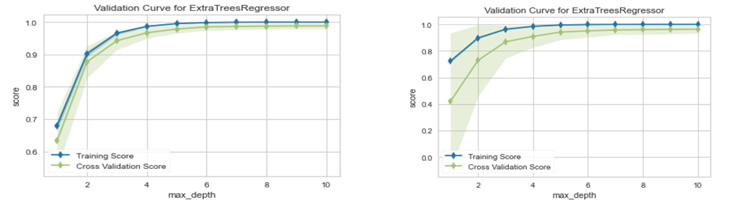
Figure 2: The learning curves of the ET model for predicting the Xi, mole fraction of N2, O2 components after 10 iterations respectively.

The learning curve provides a good insight about how the models converged for training and test samples. The small distance between train and test results in the learning curve values are another witness of avoiding overfitting in the ML models.

Conclusion

VLE of four CO2-contained binary mixtures was identified and predicted for CCS projects. ML models were trained on 70 percent of experimental data base collecting from literature and tested on the remaining 30 percent. Then PR EoS was used for prediction on the remaining 30 percent. ML produced reliable results for most of the data points with high accuracy while thermodynamic model was unable to produce results for many points with accuracy lower than ML models. It was also found out that unlike the thermodynamic model that relies on formula and critical properties of the mixture, ML relies only on pressure, temperature and relations in between the data points that makes ML faster and simpler to accommodate.

References

Hameli AF, Belhaj H, Dhuhoori AL (2022) CO2 sequestration overview in geological formations Trapping mechanisms matrix assessment. Energies 15(20): 7805.
Temitope A, Gomes JS, Bera A (2019) A review of CO2 storage in geological formations emphasizing modeling monitoring and capacity estimation approaches. Petroleum Science 16: 1028-1063.
Hematpur H, Abdollahi R, Rostami S, Haghighi M, Blunt MJ (2023) Review of underground hydrogen storage Concepts and challenges. Advances in Geo Energy Research 7(2): 111-131.
Vaferi B, Lashkarbolooki M, Esmaeili H, Shariati A (2018) Toward artificial intelligence based modeling of vapor liquid equilibria of carbon dioxide and refrigerant binary systems. Journal of the Serbian Chemical Society 83(2): 199-211.
Gokulakannan S (2022) Machine Learning And Deep Learning On Vapour Liquid Equilibrium Prediction Of Carbon Dioxide Over Amines. National Institute of Technology Rourkela.
Aminian A, ZareNezhad B (2020) A generalized neural network model for the VLE of supercritical carbon dioxide fluid extraction of fatty oils. Fuel 282(5): 118823.
Yan Y, Borhani TN, Subraveti SG, Prasad V, Rajendran A, et al. (2021) Harnessing the power of machine learning for carbon capture utilisation and storage (CCUS) a state of the art review. Energy & Environmental Science 14(12): 6122-6157.
Rahimi M, Moosavi SM, Smit B, Hatton TA (2021) Toward smart carbon capture with machine learning. Cell reports physical science 2(4): 100396.
Shih CY, Wu X (2020) A CNN-RNN based machine learning model for carbon storage management. AGU Fall Meeting Abstracts.
Truc G, Rahmanian N, Pishnamazi M (2021) Assessment of cubic equations of state machine learning for rich carbon dioxide systems. Sustainability 13(5): 2527.
Abaid AC, Svendsen HF, Jakobsen JP (2020) Surrogate modelling of VLE: integrating machine learning with thermodynamic constraints. Chemical Engineering Science X 8: 100080.
Desgranges C, Delhommelle J (2018) A new approach for the prediction of partition functions using machine learning techniques. The Journal of Chemical Physics 149(4): 044118.
Mohanty S (2006) Estimation of vapour liquid equilibria for the system carbon dioxide difluoromethane using artificial neural networks. International Journal of Refrigeration 29(2): 243-249.
Mesbah M, Soroush E, Shokrollahi A, Bahadori A (2014) Prediction of phase equilibrium of CO2/cyclic compound binary mixtures using a rigorous modeling approach. The Journal of Supercritical Fluids 90: 110-125.
Azari A, Atashrouz S, Mirshekar H (2013) Prediction the vapor liquid equilibria of CO2-containing binary refrigerant mixtures using artificial neural networks. International Scholarly Research Notices.
Bahmaninia H, Shateri M, Atashrouz S, Jabbour K, Mohaddespour A, et al. (2023) Predicting the equilibrium solubility of CO2 in alcohols, ketones, and glycol ethers Application of ensemble learning and deep learning approaches. Fluid Phase Equilibria 567: 113712.
Mehtab V, Alam S, Povari S, Nakka L, Soujanya Y, et al. (2023) Reduced Order Machine Learning Models for Accurate Prediction of CO2 Capture in Physical Solvents. Environmental Science & Technology.
Liu H, Chan VKH, Tantikhajorngosol P, Li T, Dong S, et al. (2022) Novel machine learning model correlating CO2 equilibrium solubility in three tertiary amines. Industrial & Engineering Chemistry Research 61(37): 14020- 14032.
Hwu WH, Cheng JS, Cheng KW, Chen YP (2004) Vapor liquid equilibrium of carbon dioxide with ethyl caproate, ethyl caprylate and ethyl caprate at elevated pressures. The Journal of supercritical fluids 28(1): 1-9.
Mohanty S (2005) Estimation of vapour liquid equilibria of binary systems carbon dioxide ethyl caproate, ethyl caprylate and ethyl caprate using artificial neural networks. Fluid phase equilibria 235(1): 92-98.
Roth H, Gerth PP, Lucas K (1992) Experimental vapor liquid equilibria in the systems R 22-R 23, R 22-Co2, Cs2-R 22, R 23-Co2, Cs2-R 23 and their correlation by equations of state. Fluid phase equilibria 73(1-2): 147-166.
Karimi H, Yousefi F (2007) Correlation of vapour liquid equilibria of binary mixtures using artificial neural networks. Chinese Journal of Chemical Engineering 15(5): 765-771.
Karim AMA, Mutlag AK, Hameed MS (2011) Vapor liquid equilibrium prediction by PE and ANN for the extraction of unsaturated fatty acid esters by supercritical CO2. ARPN J Eng Appl Sci 6(9): 122.
Holste JC, Hall KR, Eubank PT, Esper G, Watson MQ, et al. (1987) Experimental (p, Vm, T) for pure CO2 between 220 and 450 K. The Journal of Chemical Thermodynamics 19(12): 1233-1250.
Klimeck J, Kleinrahm R, Wagner W (2001) Measurements of the (p, ρ, T) relation of methane and carbon dioxide in the temperature range 240 K to 520 K at pressures up to 30 MPa using a new accurate single-sinker densimeter. The Journal of Chemical Thermodynamics 33(3): 251-267.
Arai Y, Kaminishi GI, Saito S (1971) The experimental determination of the PVTX relations for the carbon dioxide-nitrogen and the carbon dioxide methane systems. Journal of Chemical Engineering of Japan 4(2): 113-122.
Sarashina E, Arai Y, Sasto S (1971) The PVTX relation for the carbon dioxide argon system. Journal of Chemical Engineering of Japan 4(4): 379-381.
Davalos J, Wayne R, Anderson, Phelps RE, Kinday AJ (1976) Liquid vapor equilibria at 250.00. deg. K for systems containing methane ethane and carbon dioxide. Journal of Chemical and Engineering Data 21(1): 81-84.
Mraw SC, Hwang SC, Kobayashi R (1978) Vapor liquid equilibrium of the methane carbon dioxide system at low temperatures. Journal of Chemical and Engineering Data 23(2): 135-139.
Dorau W, Wakeel IMA, Knapp H (1983) VLE data for CO2-CF2Cl2, N2-CO2, N2-CF2Cl2 and N2-CO2- CF2Cl. Cryogenics 23(1): 29-35.
Moussa CS, Hanini S, Derriche R, Bouhedda M, Bouzidi A (2008) Prediciton of high pressure vapor liquid equilibrium of six binary systems carbon dioxide with six esters using an artificial neural network model. Brazilian Journal of Chemical Engineering 25: 183-199.
Cheng CH, Chen YP (2005) Vapor liquid equilibria of carbon dioxide with isopropyl acetate, diethyl carbonate and ethyl butyrate at elevated pressures. Fluid phase equilibria 234(1-2): 77-83.
Zarenezhad B, Aminian A (2011) Predicting the vapor liquid equilibrium of carbon dioxide+ alkanol systems by using an artificial neural network. Korean Journal of Chemical Engineering 28: 1286-1292.
Lasala S, Chiesa P, Privat R, Jaubert JN (2016) VLE properties of CO2 Based binary systems containing N2, O2 and Ar Experimental measurements and modelling results with advanced cubic equations of state. Fluid Phase Equilibria 428: 18-31.
Joung SN, Yoo CW, Shin HY, Kim SY, Yoo KP, et al. (2001) Measurements and correlation of high pressure VLE of binary CO2 alcohol systems (methanol, ethanol, 2-methoxyethanol and 2-ethoxyethanol). Fluid Phase Equilibria 185(1-2): 219-230.
Oliver GS, Luna LAG (2001) Vapor liquid equilibria near critical point and critical points for the CO2+ 1-butanol and CO2+ 2-butanol systems at temperatures from 324 to 432 K. Fluid Phase Equilibria 182(1-2): 145-156.
Oliver GS, Luna LAG, Sandler SI (2002) Vapor liquid equilibria and critical points for the carbon dioxide+ 1-pentanol and carbon dioxide+ 2-pentanol systems at temperatures from 332 to 432 K. Fluid Phase Equilibria 200(1): 161-172.
Jou FY, Otto FD, Mather AE (1998) Solubility of H2S, CO2 and their mixtures in an aqueous solution of 2-piperidineethanol and sulfolane. Journal of Chemical & Engineering Data 43(3): 409-412.
Teng TT, Mather AE (1989) Solubility of H2S, CO2 and their mixtures in an AMP solution. The Canadian Journal of Chemical Engineering 67(5): 846-850.
Li H, Jakobsen JP, Wilhelmsen O, Yan J (2011) PVTxy properties of CO2 mixtures relevant for CO2 capture transport and storage Review of available experimental data and theoretical models. Applied Energy 88(11): 3567-3579.
Westman SF, Stang HGJ, Lovseth SW, Austegard A, Snustad I, et al. (2016) Vapor liquid equilibrium data for the carbon dioxide and nitrogen (CO2+ N2) system at the temperatures 223, 270, 298 and 303 K and pressures up to 18 MPa. Fluid Phase Equilibria 409: 207-241.
Ottoy S, Neumann T, Stang HGJ, Jakobsen JP, Austegard A, et al. (2020) Thermodynamics of the carbon dioxide plus nitrogen plus methane (CO2+ N2+ CH4) system: Measurements of vapor liquid equilibrium data at temperatures from 223 to 298 K and verification of EOS- CG-2019 equation of state. Fluid Phase Equilibria 509: 112444.
Donnelly HG, Katz DL (1954) Phase equilibria in the carbon dioxide–methane system. Industrial & Engineering Chemistry 46(3): 511-517.
Esper GJ, Bailey DM, Holste JC, Hall KR (1989) Volumetric behavior of near equimolar mixtures for CO2+ CH4 and CO2+ N2. Fluid phase equilibria 49: 35-47.
Brown TS, Niesen VG, Sloan ED, Kidnay AJ (1989) Vapor liquid equilibria for the binary systems of nitrogen, carbon dioxide, and n-butane at temperatures from 220 to 344 K. Fluid phase equilibria 53: 7-14.
Djebaili K, Ahmar EE, Valtz A, Meniai AH, Coquelet C (2018) Vapor Liquid Equilibrium Data for the Carbon Dioxide (CO2)+ 1, 1, 1, 3, 3-Pentafluorobutane (R365mfc) System at Temperatures from 283.15 to 337.15 K. Journal of Chemical & Engineering Data 63(12): 4626-4631.
Hosseini M, Katragadda S, Wojtkiewicz J, Gottumukkala R (2020) Direct normal irradiance forecasting using multivariate gated recurrent units. Energies 13(15): 3914.
Jaubert JN, Mutelet F (2004) VLE predictions with the Peng Robinson equation of state and temperature dependent kij calculated through a group contribution method. Fluid Phase Equilibria 224(2): 285-304.
Hosseini M, Rostami S (2023) Project VLE, GitHub repository.

← Previous Article How Oil and Gas Companies can derive C-Factors in the API RP 14E Erosional Velocity Models for their ‘Clean Service’ Pipelines Next Article → Pressurization Characteristics and Proppants Transport of Pulse Jet Fracturing with CFD-DEM Coupling Method