Participation in the Cutting of Productive Layer Sediments of the Palchig Pilpilesi Structure to Build a 3D Geological Model of Separate Horizons and Layers to Increase the Efficiency of Field Development Analysis of Reservoir Indicators
The analysis of existing geological, geophysical researches and excavation works shows that, despite the fact that the Productive Layer (PG) sediments of the South Caspian Basin (SCB) have been the object of search and exploration for a long time, their hydrocarbon reserves have not been fully studied until now. Examination and summarization of geological-geophysical, drilling data, as well as the established 3D geological model show that the distribution of oil and gas deposits within local elevations is related to certain regularities. First of all, tectonic processes played a big role in the formation of these regularities. In the 3D geological modeling of the Palchig Pilpilesi deposit, the tectonic processes that took place in the sedimentation basin of the sedimentary complex, the development of uplifts, their complication with tectonic disturbances, and the effect of the change in the lithological composition and thickness of the horizons and layers that make up the productive layer section on the accumulation of hydrocarbon resources were considered.
Introduction
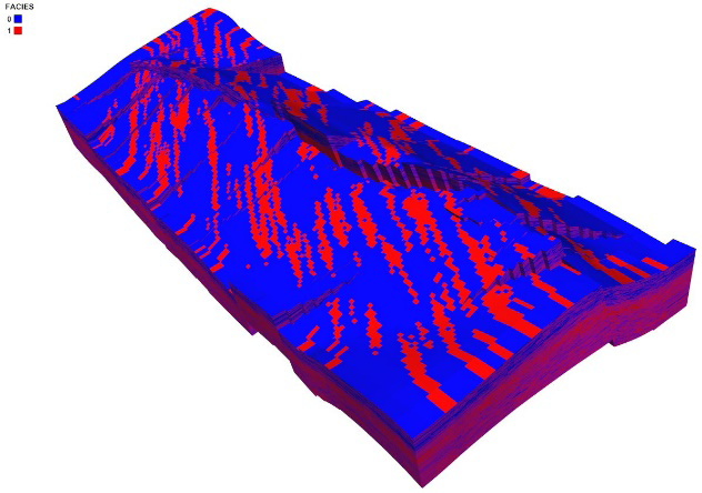
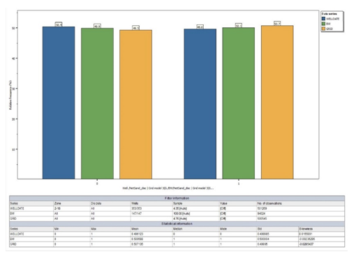
Within the construction of the 3D geological model of the deposit, the fractures surrounding the structure were modeled in 3D and a structural model was built. After verifying the structural model established by well data and trend maps, a 50x50 scale 3D grid was constructed according to the established structure, and first the seepage capacity parameter curves to be distributed by area and depth were brought to the constructed grid (BW). Facies modeling was carried out to determine the field distribution of the rocks involved in the lithological section of the development horizons. Based on the results of histogram analysis of the facies model built with the calculated parameters , we can say that the overall average value of sandiness in Palchig Pilpilesi is 0.5 across the horizons. When considered separately, it is QUG-0.26, QUQ-0.34, QD-0.36, QA-0.75 and QaLD-0.58 (Figure 1). As is known, parameters are calculated based on well data. These average values obtained were calculated based on the data within the contour. Data outside the outline has no effect on these statistics (Figure 2).
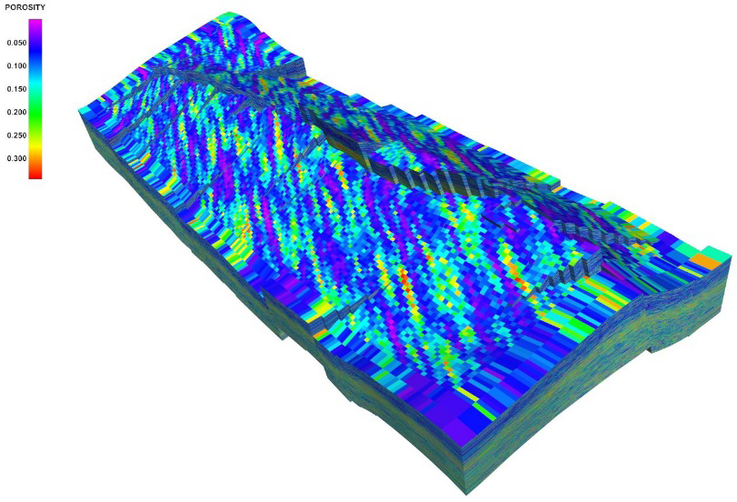
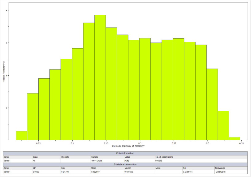
After the facies model was established, petrophysical modeling was carried out. This includes porosity, permeability and water saturation. According to the data obtained from petrophysical modeling, we can say that the average value of porosity in the horizons of the deposit is 0.183. Looking at it separately, the average value of porosity, QUG -0.19, QUQ -0.20, QD - 0.20 (QD1-0.20, QD2-0.18, QD3-0.19, QD4-0.21, QD5-0.22); QA-0.20 (QA1-0.20, QA2-0.216, QA3-0.194) and QaLD- 0.17 (QaLD1-0.17, QaLD2- 0.16, QaLD3-0.17, QaLD4- 0.18) (Figure 3).
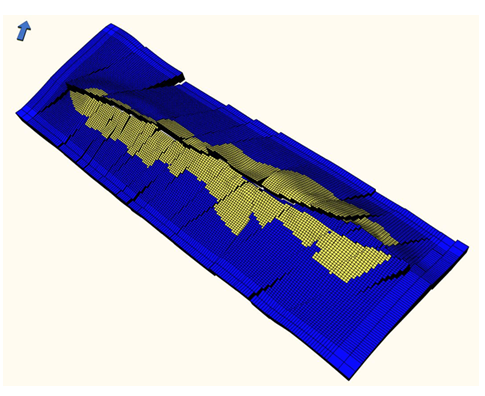
A 3D porosity (Phie) model was constructed with stochastic distribution by kriging simulation when NTG=1 (NTG=1 reservoir, NTG=0 non-reservoir) after multiple analyzes on well data.
Variogram model: Azimuth with exponential curve 170°, parallel - 150 m, normal - 100 m, vertical direction - 4 m (Figure 4).
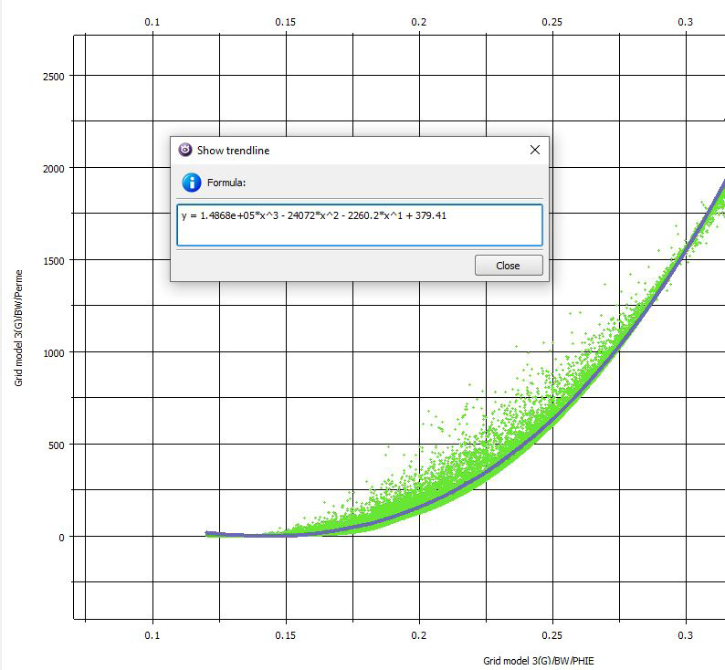
The porosity coefficient determined based on the results of the rock samples taken from the wells is based on 218 samples from 42 wells. The porosity coefficient was calculated for both horizon and bed areas. The correct calculation of the porosity coefficient by area is related to the change of the lithological composition and thickness of the reservoirs. Out of 218 samples taken from exploratory wells, 184 samples were attributed to collectors. The porosity coefficient determined for these samples varies in the range of 0.15 - 0.26. According to core analysis results and experience from other fields in the region, there is a direct relationship between permeability and porosity.
y = 1.4868e+05*x^3 - 24072*x^2 - 2260.2*x^1 + 379.41 (1)
Permeability was derived from porosity using the formula above, which reflects the increasing relationship between permeability and porosity (Figure 5).
At the next stage, the model of water saturation was established. The average value of water saturation calculated within the contour is 0.31 for the CG - QLD. If we note it with horizons, QUG is -0.33, QUQ -0.25, QD -0.35 and QA-0.28, QALD -0.32. A simplified J-function method using porosity (Poro), permeability (Perm), height above free water level (FWL) (H) and petrophysical constants (a, b) was used to model water saturation (Sw) (Figure 6).
Perm J H Poro =
1 1 d H b
= − ∫ (2)
J S H H H a top wn H top bottom bottom ( ) max w wirr w wirr wn S S S S S = + −
Swn – water saturation value by height above free water level Swirr – saturation value with non-extractable (residual) water
History Matching
Making decisions on reservoir management benefits greatly from accurate reservoir models. They can forecast reservoir performance under varied operating situations and lower the risk of investment in field development. It is essential that a reservoir model be conceptually equivalent to the reservoir in real life if it is to accurately depict the reservoir. History matching is a procedure used to evaluate and validate that the simulation model is similar to the reservoir. The reservoir’s historical performance is simulated during history-matching, and the model is modified to reflect real historical performance. It is presumable that the final history-matched model will accurately depict the reservoir and be able to forecast reservoir performance. Reducing uncertainty, enhancing reservoir understanding, validating the reservoir simulation model, and improving the accuracy of predictions of reservoir performance are the main goals and purposes of history matching reservoir models.
It is presumptively possible to forecast future performance using the reservoir model if it can accurately reproduce the reservoir’s historical performance. In order to match the model input to the recorded data, such as the fluid characteristics or the geological description, the method of “history matching” is used. Phase rates, cumulative production, pressures, tracers, temperatures, salinity, and other data can all be recorded. It will be more effective to reduce ambiguity and boost confidence in the current reservoir characterization if as much previous data can be matched. However, uncertainty can never be reduced below the uncertainty inherent in the historical data itself. In order to better comprehend the current status of the reservoir, fluid distribution, and fluid movement, as well as to confirm the current depletion mechanism, a reservoir model must be accurately historically matched. Additionally, it is feasible to learn more about operational issues such casing leaks or inefficient fluid distribution between wells (Figure 7).
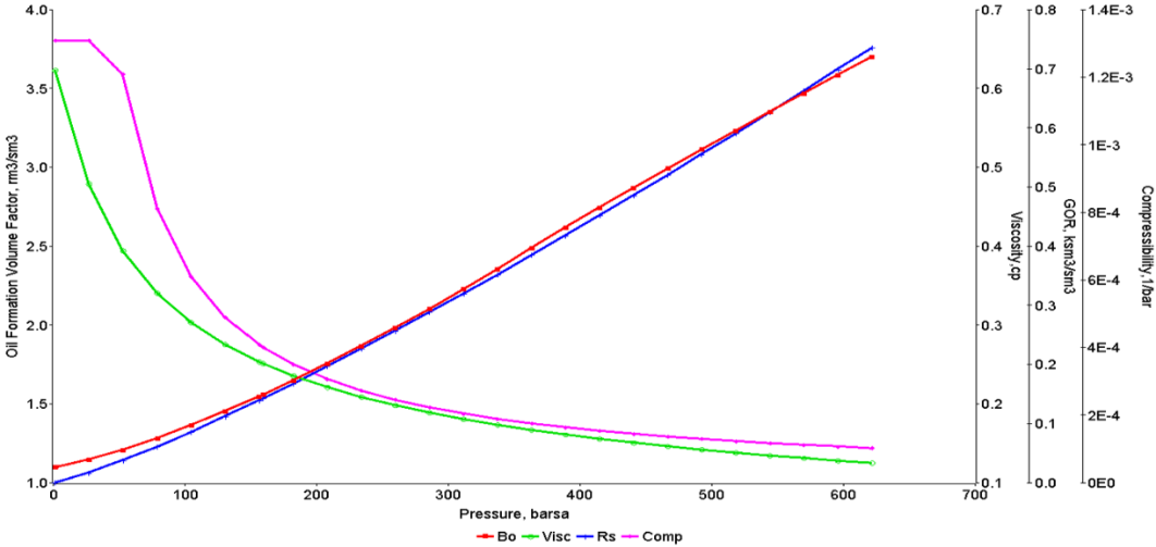
Oil PVT (Pressure-Volume-Temperature) properties refer to the characteristics of petroleum fluids under varying conditions of pressure, volume, and temperature. These properties are crucial for the exploration, production, and processing of oil and natural gas reservoirs. Here’s a brief overview of some key oil PVT properties.
Viscosity: Viscosity measures a fluid’s resistance to flow and varies with temperature and pressure. Accurate viscosity data is crucial for pipeline design and pump selection.
Compressibility: Oil’s compressibility factor indicates how much it changes in volume as pressure and temperature change. It’s important for estimating volume changes during production and injection processes.
Bubble Point and Dew Point: These critical points represent the pressure-temperature conditions at which gas begins to dissolve into or separate from the oil phase, affecting reservoir performance and phase behavior.
Saturation Pressure: Saturation pressure is the pressure at which the first bubble of gas appears in the reservoir oil. It helps in understanding the reservoir’s initial conditions.
Formation Volume Factor (FVF): FVF relates the volume of oil at reservoir conditions to its volume at surface conditions. It’s essential for converting produced volumes to standard conditions. Understanding and accurately characterizing these oil PVT properties is essential for reservoir engineering, reservoir management, and the design of oil and gas production systems. It ensures efficient and safe extraction and processing of petroleum resources (Figure 8).
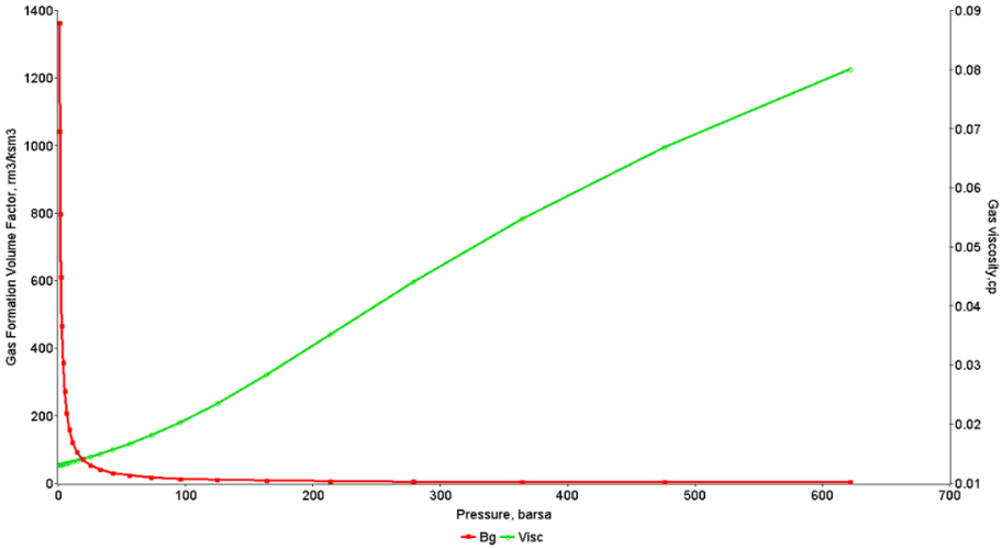
Gas viscosity and gas formation volume factor are two important properties of natural gases, and they play significant roles in various applications within the oil and gas industry. Gas viscosity refers to the resistance of a gas to flow or its internal friction as it moves. It is a measure of how easily a gas can flow through pipelines or porous reservoir rocks. Gas viscosity is a crucial parameter in pipeline design, fluid flow modeling, and reservoir engineering. It affects the pressure drop and flow rate in pipelines and influences the efficiency of gas production and transportation.
Factors Affecting Gas Viscosity: Gas viscosity is influenced by temperature and pressure. Generally, it decreases as temperature or pressure increases.
The gas formation volume factor (FVF) represents the ratio of the volume of gas at reservoir conditions (high pressure and temperature) to the volume it occupies at surface conditions (standard pressure and temperature). FVF is essential for converting measured gas volumes at surface conditions to reservoir conditions. It helps in estimating the original gas in place (OGIP) and understanding how gas behaves within a reservoir.
Factors Affecting Gas FVF: Gas FVF is primarily affected by pressure and temperature. As pressure increases, the gas becomes more compact, leading to a decrease in volume. Conversely, as temperature rises, the gas expands, increasing its volume.
Both gas viscosity and gas formation volume factor are critical for reservoir management, production optimization, and the design of efficient gas production and transportation systems. Accurate measurements and modeling of these properties are vital for ensuring the safe and cost-effective utilization of natural gas resources (Figure 9).
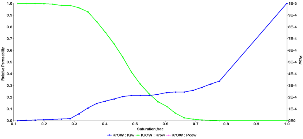
Water-oil relative permeability is a concept used in reservoir engineering and petroleum geology to describe how porous rock formations in an underground oil reservoir allow the flow of water and oil through them. Relative permeability refers to the fraction of the total permeability of the rock that is available for a particular fluid (water or oil) to flow through it.
Key Points about Water Oil Relative Permeability Relative Permeability Curve: Relative permeability is typically represented as a curve or set of curves on a graph, showing the relationship between the relative permeability of water and oil and the saturation of each fluid in the porous rock. The saturation level indicates the fraction of pore space filled with each fluid.
Saturation Levels: The relative permeability curves demonstrate how the availability of pore space for each fluid changes as the saturation levels change. The curves show that as the saturation of one fluid increases, the relative permeability of the other fluid decreases.
Understanding water-oil relative permeability is critical for optimizing oil recovery strategies in reservoir management. It guides decisions on factors such as well placement, injection of water or other fluids to displace oil, and overall reservoir development. Accurate knowledge of these relative permeability characteristics helps maximize the efficient recovery of oil while minimizing water production, which is vital for cost-effective and sustainable reservoir management (Figure 10).
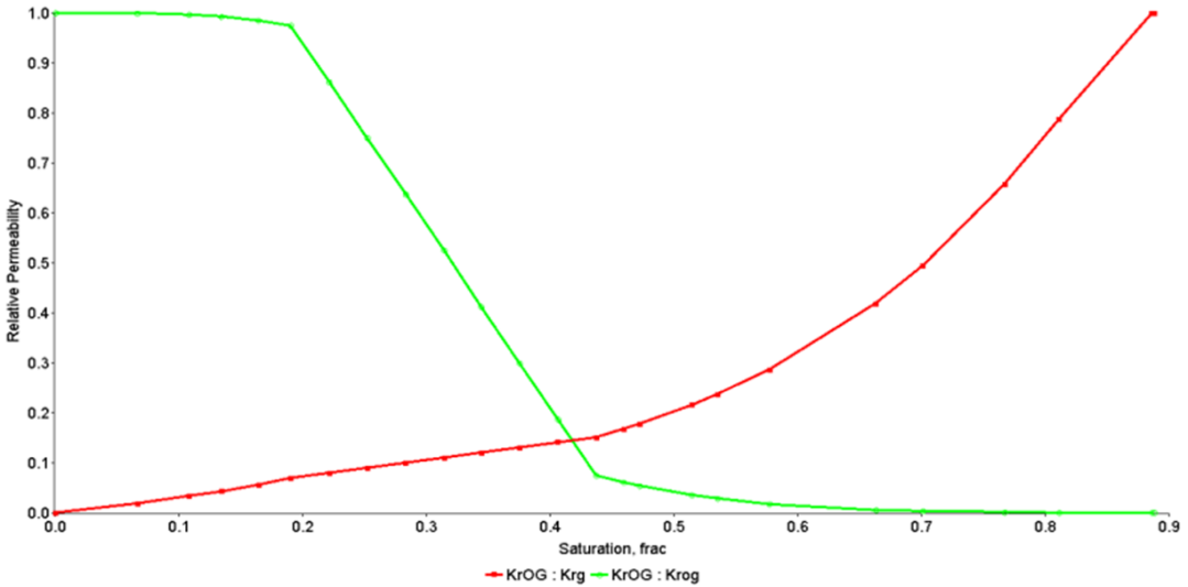
Understanding oil-gas relative permeability is essential for making informed decisions in reservoir management, particularly in situations where oil and gas coexist in the same reservoir. This knowledge helps optimize strategies for efficient hydrocarbon recovery, such as gas injection, gas cycling, and enhanced oil recovery (EOR) techniques, while minimizing unwanted gas breakthrough and ensuring economic oil production.
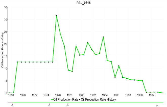
History matching is a critical process in reservoir engineering and oil production that involves adjusting the parameters of a reservoir simulation model to match observed field data, especially oil production rates, and well performance. The goal of history matching is to improve the accuracy and reliability of the reservoir model, making it a valuable tool for reservoir management and production optimization. History matching for oil production rate is a complex and time-consuming process that requires a combination of engineering expertise, reservoir modeling software, and access to accurate field data. It is a crucial step in reservoir management, as it helps in optimizing oil production, improving recovery strategies, and reducing operational costs while maintaining reservoir integrity. Figure 11 shows history matching results for well PAL_0318. History matching was achieved.
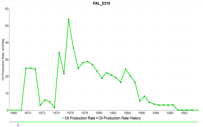
Figure 12 illustrates the outcomes of the history matching process conducted for well PAL_0319, ultimately leading to successful history matching.
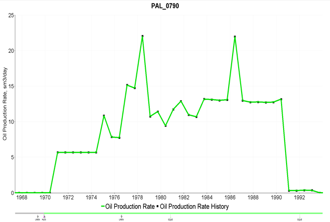
In Figure 13, we can observe the results of the history matching process specifically carried out for well PAL_0790. The successful outcome of this endeavor is evident, as the model’s predictions now closely align with the actual production data from the well. This achievement in history matching, a crucial step in reservoir engineering, signifies that the reservoir model has been meticulously adjusted to accurately represent the real-world conditions, providing a valuable tool for reservoir management and production optimization.
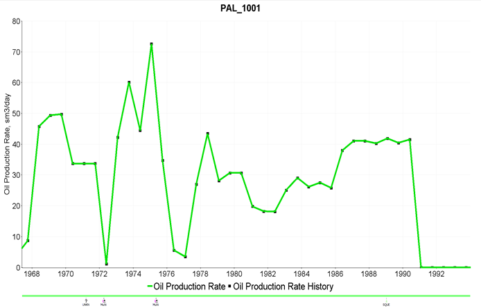
Figure 14 presents a visual depiction of the history matching process that was specifically undertaken for well PAL_1001. The results clearly reveal the successful culmination of this effort, as the model’s projections now closely mirror the observed production data emanating from the well. This successful history matching milestone, which is of paramount importance in the field of reservoir engineering, underscores the thorough and precise adjustments made to the reservoir model in order to faithfully replicate real- world conditions. As a result, the refined model now stands as a highly valuable asset, facilitating enhanced reservoir management and optimization of production processes.
There is lack of data about water aquifer for this reservoir. In order to achieve history matching, it was done some kind of sensitivity analysis for parameters of the water aquifer models and best options were selected for this reservoir model. Except thatt, it was done several lift curves for the different wells. There was information that, it were implemented various sand control methods. Due to the lack of design and parameters of the sand control methods, it was done sensitivity analysis based on the parameters of the gravel pack method and was selected optimal parameters for the reservoir model. Some of the wells were horizontal wells. But, there weren’t trajectories of these wells and data about their horizontal section. Based on this research, it was done sensitivity analysis to define optimal length of the horizontal section for these wells. Same process was implied for gas-lift wells. There weren’t exact volume of gas-lift gas injection volume and therefore, several cases were generated to determine the suitable gas-lift gas injection volume. Optimization of wells were done and it helps to find optimal gas-lift gas injection volume.
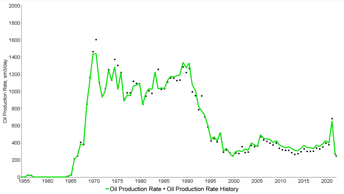
Figure 15 shows as a visual representation of the outcomes derived from the endeavor to match the oil field’s production rates. In the subsequent stages of the process, notably for predictive purposes, the critical milestone of history matching must be attained. This integral step involves aligning the reservoir model with actual production data, ensuring that it faithfully mirrors real-world conditions. It is only upon successfully achieving history matching that the model becomes a dependable tool for forecasting and optimizing production processes within the oil field.
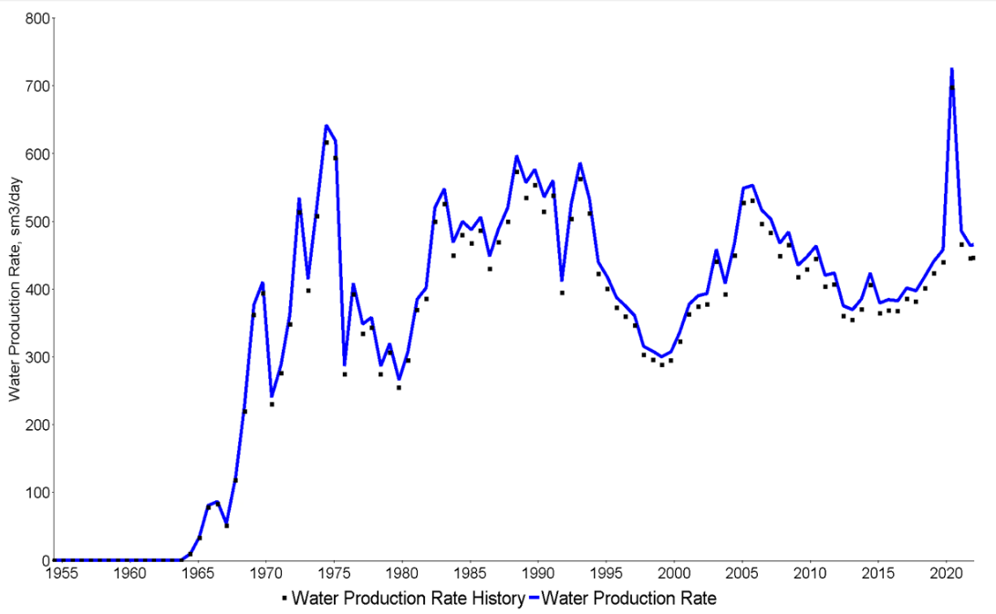
Figure 16 represents the results for matching of water field production rate. For further process, to do prediction, history matching must be achieved.
Conclusion
For the first time, a 3D geological model of the Mud Pilpilesi deposit was built using the RMS software package of the ROXAR company. For this, a database of the field was initially created, and a structural model covering the horizons under development (QUG, QUQ, QD1, QD2, QD3, QD4, QD5, QA1, QA2, QA3, QaLD1, QaLD2, QaLD3, QaLD4) was built. A 3D network (grid) was established by clarifying the fault blocks formed during tectonic processes, facies and petrophysical modeling were performed, and as a result, the initial balance hydrocarbon reserve of the field was calculated. The 3D geological grid was “upscaled” to the hydrodynamic grid for the purpose of forecasting the application of various methods for restoring the history and increasing the processing efficiency. In order to determine the degree of influence of the parameters in the calculation of the initial balance hydrocarbon reserve, sensitivity analysis and the study of the effect of uncertainties have been performed. History match was done by determining the optimal horizontal section for horizontal wells, by finding the optimal gas-lift gas injection volumes, by determining the gravel pack parameters and by defining the parameters of the water quifer models.
References
-
Baker RO, Chugh S, Mcburney C, Mckishnie R (2006) History Matching Standards Quality Control and Risk Analysis for Simulation. International Petroleum Conference, pp: 13-15.
-
Caers J (2005) Petroleum Geostatistics. Society of petroleum engineers, pp: 104.
-
Jabrayil E (2021) Effectiveness of the well drainage area by changing horizontal well section. Azerbaijan Oil Industry Journal, pp: 26-29.
-
Kabir CS, Young NJ (2001) Handling production-data uncertainty in history matching The Meren reservoir case study. SPE Annual Technical Conference and Exhibition.
-
Carlson MR (2006) Practical Reservoir Simulation. PennWell Corporation, pp: 516.
-
Eyvazov J, Guliyeva M (2023) Increase Oil Recovery in Different Surfactant Concentrations on the Basis of Increasing Well Drainage Area. Progress in Petrochemical Science 5(1): 464-467.
-
Jafarpour B, McLaughlin DB (2007) History matching with an Ensemble Kalman filter and discreate cosine parameterization. SPE Annual Technical Conference and Exhibition, pp: 11-14.
-
Aanonsen SI, Aavatsmark I, Barkve T, Cominelli A, Gonard R, et al. (2003) Effect of Scale Dependent Data Correlations in an Integrated History Matching Loop Combining Production Data and 4D seismic Data. SPE Reservoir Simulation Symposium, pp: 3-5.
-
Eyvazov J, Guliyeva M, Guliyev U (2022) How the Oil Recovery Factor Changes in Different Polymer Concentrations on in the Basis of Increasing Well Drainage Area. International Petroleum and Petrochemical Technology Conference. Springer, Singapore, pp: 133- 140.
-
Kleppe J (2008) Reservoir simulation lecture note 4 and 6. Norwegian University of science and technology. NTNU, Norway.
-
Lepine OJ, Bissell, RC, Aanonsen SI, Pallister I, Barker JW (1998) Uncertainty analysis in predictive reservoir simulation using gradient information. SPE Annual Technical Conference and Exhibition, pp: 27-30.
-
Eyvazov J, Hamidov N (2023) The Effect of Different Hydraulic Fracturing Width to the Well Production. International Journal of Oil Gas and Coal Engineering 11(4): 74-78.
-
Mattax CC, Dalton RL (1991) Reservoir simulation. Journal of Petroleum Technology 42(6): 692-695.
-
Li R, Reynolds AC, Oliver DS (2003) History matching of three-phase flow production data. SPE Journal 8(4): 328-340.
-
Eyvazov J, Hamido N (2023) The effect of hydraulic fracturing length to the well production. Journal of Physics Conference Series 2594(1): 012022.
-
Bissell R (1994) Calculating optimal parameters for history matching. 4th European Conference on the Mathematics of Oil Recovery, European Association of Geoscientists & Engineers.
-
Dougherty EL, Khairkhah D (1975) History Matching of Gas Simulation Models Using Optimal Control Theory. SPE California Regional Fall Meeting, pp: 2-4.
-
Eyvazov J, Guliyeva M, Guliyev U (2022) The Effect of Sand Production to the Well Drainage Area. Proceedings of the 2022 International Petroleum and Petrochemical Technology Conference, Springer, Singapore, pp: 141- 146.
-
Harb R (2004) History matching including 4D seismic An application to a field in the North Sea. Master thesis NTNU Norway.
-
Nocedal J, Wright SJ (1999) Numerical Optimization. 2nd(Edn.), Springer Series in Operations Research and Financial Engineering. Springer New York, NY, pp: 1012.
-
Eyvazov J (2022) Sensitivity analysis of oil and gas production as a result of increasing the drainage area within changes in well parameters during different completion of wells. SOCAR Proceedings 2: 019-022.
-
Shah PC, Gavalas GR, Seinfeld JH (1978) Error analysis in history matching: the optimum level of parameterization. Soc Petrol Eng J 18(6): 219-228.
- Nigeria’s Vulnerability in the Face of Global Energy Policy
- A Simulation Study of Investigation of Optimum Oil Production Performance by Applying Various Gas Injection Methods in Oil Reservoir
- Characterization of Permo-Triassic Reservoirs through Thermal Maturity Assessment of Westphalian Source Rocks in the Cheshire Basin
- Influence of Microwax on the Rheological and Thermal Behaviour of a Wax Crude Oil
- Real-Time Monitoring and Performance Optimization of Steam Injection in Heavy Oil Reservoirs Using Fiber Optic Sensing and Integrated Predictive Simulation Models
- Rapid On-Site Determination of the Total Petroleum Hydrocarbon Content of Soils by Handheld Fourier Transform Near-Infrared Spectroscopy: Development of a Global, Site- and Scanner- Independent Calibration Model