Numerical Simulation of a Multilateral Saturated Reservoir using MATLAB-based Simulator
This paper presents a detailed numerical simulation study of a multilateral saturated reservoir using a MATLAB-based simulator. The study focuses on the calculation of various parameters such as pressure, temperature, flow regime, gas and oil velocity, and pressure drops. The simulator uses four MATLAB script files and five function files to perform these calculations. The simulation results are analyzed and presented in various graphs and charts, including pressure vs depth, temperature vs depth, flow regime vs depth, gas and oil velocity vs depth, delta pressures vs depth, mixture density vs depth, liquid holdup vs depth, and production rates. In addition to presenting the simulation results, the study also conducts sensitivity analyses to examine the effects of varying wellhead pressure, reservoir thickness, and reservoir permeability. The sensitivity analyses provide useful insights into how changes in these parameters can affect the behavior of multilateral saturated reservoirs. Overall, the study concludes that the MATLAB-based simulator provides an effective tool for analyzing the behavior of multilateral saturated reservoirs. The simulator can be further improved by incorporating additional features and functionalities. The findings of this study can be useful for reservoir engineers and other professionals in the oil and gas industry who are involved in the design and optimization of production systems for multilateral saturated reservoirs. In summary, this paper contributes to the existing body of knowledge on numerical simulation of multilateral saturated reservoirs and provides a valuable resource for researchers and practitioners in the field.
Ekrem Alagoz¹*, Emre Can Dundar¹ and Mouad Al Krmagi²
¹Turkish Petroleum Corporation (TPAO), Turkey ²Texas A&M University, USA
resource for researchers and practitioners in the field.
Introduction
In the realm of oil reservoir engineering, the effective exploitation of multilateral oil wells presents a challenging yet pivotal endeavour. These wells, characterized by their intricate geometries and diverse flow dynamics, often harbour complex production systems with unique operational considerations. Within this context, our study delves into the nuanced interplay between reservoir characteristics, well geometry, and production performance. At the heart of our investigation lies the configuration of a multilateral oil well, where two non-communicating layers within the reservoir dictate the flow dynamics. The well structure comprises horizontal, curvic, and vertical sections, each exerting its influence on the fluid flow behavior. Our endeavor is propelled by the imperative to develop a robust numerical simulator, drawing upon the foundational models proposed by Orkiszewski and Vogel [1].
The primary objective of our study is threefold: firstly, to construct a numerical framework capable of elucidating various flow regimes encountered within the production system. Secondly, to leverage this simulator to compute essential parameters such as pressure drop, liquid holdup, mixture density, and velocities of gas and oil along the wellbore. Lastly, to extrapolate valuable insights into gas and liquid production rates, thus enabling a comprehensive understanding of the system’s performance characteristics. To exemplify the utility of our numerical simulator, we embark on a practical demonstration, simulating a specific production system under defined wellhead pressures [2]. Through meticulous analysis, we scrutinize the spatiotemporal distribution of pressure drop, liquid holdup, mixture density, and velocities along the length of the well. Furthermore, we delve into the intricacies of flow regimes, discerning the significance of potential, kinetics, and frictional pressure drops on the overall system behavior [3]. Subsequently, our inquiry extends to a sensitivity analysis, where we systematically diversify well properties and production rates in response to changes in wellhead pressure. This comprehensive examination not only underscores the adaptive capacity of the production system but also illuminates critical operational considerations in optimizing production strategies. In summation, our study endeavors to unravel the complexities inherent in multilateral oil well systems, offering a nuanced understanding of their performance dynamics. By harnessing the power of numerical simulation and rigorous analysis, we aim to furnish reservoir engineers with indispensable tools for enhancing operational efficiency and maximizing production yields in multilateral oil well environments.
The efficient extraction of hydrocarbons from natural gas formations hinges on accurate production forecasting and a profound understanding of pressure dynamics within gas wells. In this context, the present study addresses the intricate interplay between transient flow behavior and pressure drop phenomena to facilitate optimized gas production strategies. There is also a detailed research of the mathematically modelling a hydrocarbon shale reservoir with the natural fractures, and its impacts on the well completion and stimulation processes –specifically hydraulic fracturing processes- are analyzed., and the study is applied for five most important US shale reservoirs [4].
In-depth research has delved into the dynamics of pressure distribution within pore throats, with a focus on elucidating the fundamental mechanisms governing fluid flow in porous media. Alagoz and Giozza conducted a sensitivity analysis on bottomhole pressure calculations in two-phase wells, providing valuable insights into the factors influencing pressure dynamics within such systems [5]. Furthermore, Alagoz, et al. [5] have contributed to the field by developing computational tools for analyzing wellbore stability, thereby enhancing our understanding of pressure behavior in complex geological formations [6]. These studies have laid the groundwork for comprehending pressure dynamics in pore throats and have paved the way for further exploration in this area.
Previous Works
Amin, et al. [7] discuss the rising norm of drilling multi- lateral wells for enhanced reservoir coverage, improved productivity, and better financial returns. Their study introduces a multi-parametric optimization approach for designing and placing multi-lateral wells to maximize contact with productive hydrocarbon zones. Utilizing advanced 3D transient numerical models that incorporate dynamic data, the study simulates transient-pressure behaviors of multi- lateral wells accurately. The optimization process considers variables such as the number of laterals, spacing, and lateral length based on reservoir characteristics, generating multiple well patterns to identify the most productive configuration. Ahmet et al. emphasize minimizing competition among laterals and maximizing the drainage area, which is crucial for optimizing productivity, especially in permeable and tight reservoirs. They present graphical productivity indices from these simulations to guide the selection of the best well design. Additional sensitivity analyses illustrate the impact of reservoir heterogeneity, lateral length, spacing, and the presence of offset producers or injectors. Their workflow has been successfully tested and aids in designing optimal multi- lateral wells for various reservoir conditions.
Alagoz and Dundar [8] provide a comprehensive analysis of gas well production forecasting and pressure dynamics within natural gas formations. By focusing on transient flow conditions and assuming Darcy flow with zero skin factor, the authors investigate two key aspects: production forecasting and pressure drop analysis. Their primary objective is to develop a production forecast until the average reservoir pressure declines to 2,000 psi. Additionally, the paper delves into the pressure drop along the well, detailing its components such as friction, acceleration, and gravitational potential, with depth profiles presented for at least one average reservoir pressure scenario. Moreover, temporal variations in pressure drop are considered, offering insights into the evolution of these dynamics over time. Through rigorous examination and discussion, this study contributes valuable insights for optimizing gas well production strategies and enhancing understanding of pressure behavior in natural gas formations Aranguen, et al. [9] explore cutting-edge sequence-based machine learning models, commonly used in language processing, to reproduce a multi-porosity reservoir simulator. Their approach integrates advanced techniques to significantly reduce numerical simulation time and improve decision-making for Huff and Puff (H-n-P) gas injection optimization in shale reservoirs. The method involves three crucial steps: 1) validating simulation results against actual data, 2) training and validating a machine learning model using simulation results from commercial or in-house numerical simulators, and 3) exhaustively exploring hyperparameter tuning and selecting machine learning techniques, such as sequence-to-sequence (Seq2Seq), Luong attention, and ConvLSTM. The proxy model uses well control parameters— like injection and production periods, number of cycles, and gas injection rates—as input variables to estimate results. This multi-porosity proxy reservoir simulation model combines numerical simulation with data-driven techniques [10]. Despite the significant time required for tuning the model, it can speed up simulation time by up to 20,000 times, enabling the generation of hundreds or thousands of scenarios within minutes, albeit with some reduction in accuracy. Notably, with a small training dataset, the proxy model can accurately predict oil production in complex low and ultra-low permeability reservoirs, significantly reducing error relative to the multi-porosity reservoir simulator. The ability to reproduce numerous scenarios quickly allows for the exploration of different well control configurations. The novelty of this proxy multi-porosity reservoir simulator lies in its ability to accelerate numerical simulation time by using techniques that solve sequence learning problems where outputs depend on previous outputs. Alagoz E, Dundar EC [11, 12] conducted a comprehensive comparative analysis of gas production forecasts for non-fractured and fractured vertical gas wells. By examining factors such as Darcy flow, zero skin factor assumptions, and fracture stimulation techniques, the study highlights the significant impact of fracture stimulation on enhancing gas recovery rates and overall profitability. The findings demonstrate substantial differences in production volumes and economic outcomes across various fracture program models, underscoring the importance of strategic decision-making in optimizing resource utilization and maximizing revenue. This research elucidates the interplay between reservoir characteristics, operational parameters, and economic considerations, providing a valuable framework for guiding future research and industry practices. The insights gained are crucial for informing stakeholder decisions and advancing gas production technologies and strategies.
In the realm of unconventional well production forecasting, Laalam, et al. [13] conducted a comprehensive evaluation of empirical correlations and time series models, focusing on the Wolfcamp A Formation. Their study compared the performance of traditional decline curve models with advanced machine learning techniques such as ARIMA, LSTM, and GRUs. The research highlighted that no single model consistently excelled across all scenarios, emphasizing the necessity for tailored approaches based on specific reservoir characteristics. Notably, the ARIMA model demonstrated superior accuracy with an R2-score of 93.50%, outperforming the Logistic Growth Model. This underscores the potential of advanced statistical methods and machine learning models in managing the complex data typical of unconventional reservoirs [13]. In a related study, Dehdouh, et al. [14] explored the application of Fishbone Drilling (FbD) technology to enhance recovery efforts in the Bakken formation. Their investigation revealed that FbD, characterized by multiple minor holes branching from the main wellbore, significantly improves hydrocarbon recovery by enhancing reservoir contact and exploiting natural fractures more effectively than traditional methods. The study’s detailed numerical simulations and comparative analyses highlighted the superior performance of FbD over conventional drilling and fracturing methods, suggesting a promising avenue for future exploration and development within unconventional reservoirs [14]. Our study builds upon these findings by implementing a MATLAB-based simulator to analyze multilateral saturated reservoirs. This approach involves detailed numerical simulations that calculate critical parameters such as pressure, temperature, flow regime, and production rates, providing a robust framework for sensitivity analyses and optimization in reservoir management.
Relevant Dimensions, Properties, and Assumptions
In the present study, a comprehensive examination of the properties outlined in the original problem statement is facilitated through tabulation in the accompanying table. It is noted that the productivity indices provided in the problem statement were omitted from integration into the simulator owing to compatibility concerns. This decision was made to ensure the robustness and reliability of the simulator’s functionality in addressing the core objectives outlined in the research (Tables 1 & 2, Figure 1).
| Well Properties | ||
|---|---|---|
| Tubing inner Diameter (in) | 3 | |
| Pipe Roughness (in) | 0.002 | |
| Wellhead temperature (oF) | 115 | |
| Lateral No | 1 | 2 |
| Interval length, L (ft) | 500 | 5200 |
| Radius of curve, R (ft) | 300 | 300 |
| Reservoir Properties | ||
| Bottomhole temperature (T, oF) | 230 | 210 |
Table 1: Well and Reservoir Properties used as an Input for this Study.
| Property | Value |
|---|---|
| Temperature (T) | 210°F |
| Pressure (Pi) | 4400 psi |
| Oil Density (GammaO) | 32° API |
| Gas Density at Separation (GammaGS) | 0.71 |
| Bubble Pressure (Pbub) | 4300 psi |
| Irreducible Water Saturation (Srw) | 0.25 |
| Pressure at Separation (Psep) | 114.7 PSI |
| Wellbore Radius (rw) | 1 inch |
| Temperature at Separation (Tsep) | 75°F |
| Reservoir Thickness (h) | 100 feet |
| Reservoir Permeability (k) | 5 (no anisotropy) |
| Reservoir Length (twoxe) | 500 feet |
| Reservoir Width (twoye) | 1000 feet |
Table 3: Properties of Upper Formation.
These properties serve as fundamental inputs for the numerical simulation and analysis conducted in this research endeavor, contributing to the comprehensive characterization of the multilateral oil well system under investigation (Table 3).
These properties are instrumental in the analysis and modeling of Formation 2 within the multilateral oil well system, contributing to a comprehensive evaluation of its behavior and performance. In the development of the simulator tailored for the multilateral oil well scheme, it is imperative to acknowledge the inherent nature of approximations inherent in such modeling endeavors. These approximations serve to streamline the complexity of the problem domain, facilitating a more tractable analytical framework. Within this context, several key assumptions were integrated into the simulator to enhance its computational efficiency and practical applicability. These assumptions encompass:
| Property | Value |
|---|---|
| Temperature (Ttwo) | 230°F |
| Pressure (Pitwo) | 4500 psi |
| Pressure at Wellbore Entry (Pwftwo) | 4300 psi |
| Oil Density (GammaO) | 32° API |
| Gas Density at Separation (GammaGS) | 0.71 |
| Bubble Pressure (Pbub) | 4300 psi |
| Irreducible Water Saturation (Srw) | 0.2 |
| Pressure at Separation (Psep) | 114.7 PSI |
| Temperature at Separation (Tsep) | 75°F |
| Wellbore Radius (rw) | 1 inch |
| Reservoir Thickness (htwo) | 100 feet |
| Reservoir Permeability (ktwo) | 5 (no anisotropy) |
| Reservoir Length (twoxe) | 5200 feet |
| Reservoir Width (twoye) | 1000 feet |
Table 2: Properties of Lower Formation.
Vogel Assumption on Wellbore Pressure: The simulator operates under the assumption that the wellbore pressure remains at or below the bubble pressure throughout the production process. This assumption aligns with Vogel’s model, facilitating a simplified representation of pressure behavior within the wellbore. Selective Perforation on Horizontal Sections: Perforation operations are constrained to the horizontal segments of the well. This selective perforation strategy optimizes the efficiency of fluid extraction from the targeted reservoir zones, while also simplifying the computational complexity associated with modelling perforation effects.
Zero Skin Factor: A skin factor of zero is assumed throughout the simulation process. This assumption negates the presence of any formation damage or completion inefficiencies, thereby streamlining the estimation of flow parameters and enhancing the computational feasibility of the model. Infinite Conductivity along Horizontal Sections: Along the horizontal sections of the well, infinite conductivity conditions are presumed. This idealized scenario enables a straightforward representation of fluid flow dynamics, neglecting any impedance to flow within the reservoir matrix.
Pseudo-Steady State Operating Condition: The simulation operates under the assumption of pseudo-steady state conditions. This assumption implies that the production system exhibits a quasi-equilibrium state, with fluid flow rates and pressure distributions evolving slowly over time compared to the timescale of interest. By incorporating these physical assumptions into the simulator framework, a pragmatic balance is struck between computational tractability and fidelity to real-world operating conditions. While these assumptions inherently introduce simplifications, they nevertheless facilitate a robust analytical tool for evaluating the performance of multilateral oil well systems and informing decision-making processes within the realm of reservoir engineering.
Solution Approach
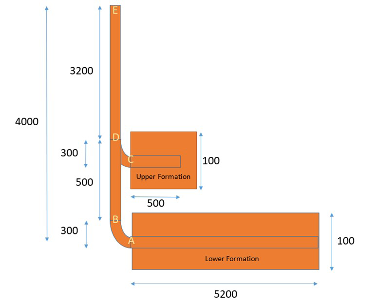
The simulator works from the bottom of the well reservoir system and calculate appropriate values as depth decreases (moving up the well); and, finally reaching the wellhead. At horizontal well number 2 (lower formation), a wellbore pressure is assumed. As stated in the assumption, this wellhead pressure must be at or below bubble point of the reservoir fluid. The reservoir pressure is assumed to be above bubble point. The simulator then calculates the production rates of gas and oil at local pressure and temperature (point A on the production system diagram). Using these values, the simulator calculates the pressure drop along the curve section of well number 2.
The curve section is divided into 6 section of equal elevation change (50ft). Along the way, the simulator updates the flow rates and fluid properties of oil and gas. At the end of the curve section (point B on the production system diagram), the simulator calculates the pressure drop along the vertical section of well number 2. This vertical section is divided into sections of equal length (100ft). Along the way, the simulator updates the flow rates and fluid properties of oil and gas.
At the end of the vertical section of well number 2, the pressure is marked. Then the simulator finds an appropriate production rate of well number 1 (by adjusting wellbore pressure); such that, the pressure at the end of curve section of well number 1 matches the pressure at the end of the vertical section of well number 2 (point D on the production system diagram). This operation is done by iteration with error tolerance of 0.05%. Once the pressures converge, the total fluid velocities were calculated by values originating from wells 1 and 2. Then, the simulator calculates the pressure drop along the final vertical section of the well, all the way to the surface. This vertical section is divided into sections of equal length (100ft). Like previous methods, the simulator also updates the flow rates and fluid properties of oil and gas along the way. At wellhead, production values of oil and gas are given in barrel/day calculated at wellhead pressure and temperature.
Equation of state for oil density (Vazquez and Beggs [15])
This model is used to update the density of oil at the end of each calculation interval. F = (Ttwo-60)*GammaO/GammaGS; A1 = GammaO/(Ttwo+460); Rs = GammaGS*Pitwo^1.187/56.06*10^(10.393*A1); Bob = 1+4.67*10^(-4)*Rs+0.11*10^(-4)*F+0.1337*10^(-8)*Rs*F; rhol = ((141.5/(GammaO+131.5))+ 2.179*10^-4*GammaGS*Rs)/ Bob; %Oil density in g/cm3
Viscosity model for oil below bubble pressure
This model is used to update the density of oil at the end of each calculation interval. a = 10.715*(Rs+100)^-0.515; b = 5.44*(Rs+150)^-0.338; C2 = 3.0324-0.02023*GammaO; B2 = 10^C2; A2 = B2*Ttwo^-1.163; miuod = 10^A2-1; miuob = a*miuod^b;
Saturated reservoir production model at pseudo-steady state (Vogel)
This model is used to determine the production of oil and gas from a saturated reservoir using a horizontal well. The maximum oil production rate is a modified Babu and Odeh model for saturated reservoir taken from Economides production engineering textbook. This model assumes a rectangular reservoir. The length of the reservoirs is set equal to the lengths of wells for simplified calculation. The rate of gas production is calculated using Rs factor (the amount of gas separated from oil under certain separation conditions) in addition to the gas produced at the wellbore. qo = (1-0.2*(Pwftwo/Pitwo)-0.8*(Pwftwo/ Pitwo)^2)*qmaxo qg = (1-0.2*(Pwftwo/Pitwo)-0.8*(Pwftwo/Pitwo)^2)*qmax g+(Rs*qo*Bob)*Bg/5.61458333; lnCH = 6.28*twoye/htwo*(1/3-(0.5)+0.5^2)-log(sin(pi/2))- 0.5*log(twoye/htwo)-1.088; qmaxo = ktwo*kro*twoxe*Pitwo/(254.2*miuob*(log(((twoy e*htwo)^0.5)/rw)+lnCH-0.75)); qmaxg = ktwo*krg*twoxe*Pitwo/(254.2*miug*(log(((twoye *htwo)^0.5)/rw)+lnCH-0.75));
Equation of state for gas density (Brill and Beggs [16])
This model is used to update the density of gas at the end of each calculation interval.
Tpc = 390; %Critical temperature in Rankin
Ppc = 665; %Critical pressure in psi
Tpr = (T+459.67)/Tpc;
Ppr = P/Ppc;
E = 9*(Tpr-1);
F = 0.3106-0.49*Tpr+0.1824*Tpr^2;
A = 1.39*(Tpr-0.92)^0.5-0.36*Tpr-0.1;
$$ \begin{array}{l} B = (0. 6 2 - 0. 2 3 * T p r) ^ {*} P p r + (0. 0 6 6 / (T p r - 0. 8 6) - \\ 0. 0 3 7) ^ {*} P p r ^ {2} + 0. 3 2 ^ {*} P p r ^ {6} / 1 0 ^ {\mathrm {E}}; \\ \end{array} $$
C = 0.132-0.32*log10(Tpr);
D = 10^F;
z = A+(1-A)/exp(B)+C*Ppr^D;
rhog = 28.967*GammaGS*(Ptubing*6894.76)/(z*8314*(((Tt
ubing-32)/1.8)+273.15));
%Gas density in kg/m3
Equation of state for gas viscosity (Lee,Gonzalez, Eakin [17])
This model is used to update the viscosity of gas at the end of each calculation interval. A3 =(9.379+0.01607*16.04)*(Ttwo+459.67)^(1.5)/(209.2+ 19.26*16.04+(Ttwo+459.67)); B3 = 3.448+986.4/(Ttwo+459.67)+0.01009*16.04; C3 = 2.447-0.224*B3; miug = A3*(10^(-4))*exp(B3*(rhog/1000)^(C3));
Flow regime determination for two-phase flow in tubing (Orkizewski)
This model is used to determine the flow regime at each calculation interval. Regimes 1,2,3,4 are bubble flow, slug flow, transition flow, and mist flow, respectively. qt = qo+qg; ut = qt/6.289811/(24*60*60)/TubeA; %Total fluid velocity in m/s ug = qg/qt*ut; %Gas velocity in m/s ul = qo/qt*ut; %Oil velocity in m/s psi = 1.071-(0.7277*ut^2/(TubeD*0.0254)); if psi < 0.13 psi = 0.13; end gravity = 981; Sigma = 37.5-0.2571*GammaO; Nlv = ul*(rhol/(gravity*Sigma))^0.25; Ngv = ug*(rhol/(gravity*Sigma))^0.25; Rgl = ug/ul; if ug/ut < psi regime = 1; else if Rgl*Nlv < (50+36*Nlv) regime = 2; end if (50+36*Nlv) < Rgl*Nlv && Rgl*Nlv <(75+84*Nlv^0.75) regime = 3; end if Rgl*Nlv > (75+84*Nlv^0.75) regime = 4; end end
Pressure Drop Model along Tubing (Orkizewski)
This model is used to determine the pressure drop components (potential and frictional) along each calculation interval. The calculation for kinetic pressure drop is done separately after updating the equation of states for oil and gas at the end of the interval. Note, that this approach assumes minimal contribution of frictional pressure loss. This assumption will be justified later in the report. Additionally, the model is only designed for bubble and slug flow regimes. This decision was made after observing that the flow regimes never entered transition or mist flows anywhere along the well under varying reservoir conditions and wellhead pressures.
if regime == 1 %Pressure drop calculation if bubble flow um = ut; yg = 0.5*((1+um/0.24)-((1+um/0.24)^2- (4*ug/0.24))^0.5); rhom = yg*rhog+(1-yg)*rhol*1000; chi = rhom*um*ug/(Ptubing*6894.76); GPDelta = (rhom*9.81*(ElevationChan ge*0.3048)*0.000145038)/(1-chi); %Potential pressure drop in psi per 50 ft Re = TubeD*0.0254*rhol*1000*ul/(miuob*10^-3); if Re < 2100 ff = 16/Re; else ff = ((-2*log10(epsil/(3.7065*TubeD)-5.0452/ Re*log10(1/2.8257*(epsil/TubeD)^1.1098+5.8506/ Re^0.8981)))^-1)^2; end FPDelta = (2*ff*ul^2*(rhol*1000)/
(TubeD*0.0254)*0.000145038)/(1-chi)*Length*0.3048; %Friction pressure drop in psi per 50 ft KPDelta = 0; %Kinetic pressure drop assumed negligible. To be calculated later. end if regime == 2 %Pressure drop calculation if slug flow vsguest = ug-ul; Nregs = TubeD*0.0254*rhol*1000*abs(vsguest)/ (miuob*10^-3); Nret = TubeD*0.0254*rhol*1000*abs(ut)/ (miuob*10^-3); CGW3 = 0.35; CGW4 = 0.17/6000*Nret+1; us = CGW3*CGW4*(9.81*TubeD*0.0254)^0.5; syms x yg = vpasolve([ug/x-ul/(1-x) - us == 0],[x]); yg = yg(1); rhomGW = rhol*1000*(ul+us)/(ul+ug+us); if ut < 3; n = 1.415; a1 = 2.364*10^-3; a2 = -0.140; a3 = 0.167; a4 = 0.113; a5 = 0; else n = 1.371; a1 = 5.375*10^-3; a2 = 0.455; a3 = 0; a4 = 0.569; a5 = -(0.516+log10(ut))*(1.547*10^- 3*log10(miuob+1)/(TubeD*0.0254)^1.571+0.722+0.63*log 10(TubeD*0.0254)); end Gamma = a1*log10(1000*miuob*10^-3)/(TubeD* 0.0254)^n+a2+a3*log10(ut)+a4*log10(TubeD*0.0254)+a5; rhomO = rhomGW+Gamma*rhol; GPDelta = (rhomO*9.81*(ElevationChan ge*0.3048)*0.000145038); %Potential pressure drop in psi per 50 ft Re = TubeD*0.0254*rhol*1000*ut/(miuob*10^-3);
if Re < 2100 ff = 16/Re; else ff = ((-2*log10(epsil/(3.7065*TubeD)-5.0452/ Re*log10(1/2.8257*(epsil/TubeD)^1.1098+5.8506/ Re^0.8981)))^-1)^2; end FPDelta = (2*ff*ut^2*(rhomO)/(TubeD*0.0254)*0.0 00145038)*Length*0.3048; %Frictional pressure drop in psi per 50 ft KPDelta = 0; %Kinetic pressure drop assumed negligible. To be calculated later. end if regime == 1 rhomix = rhom; else rhomix = rhomO; end
About Simulator
The simulator for this production system is done on Matlab. The code is divided into four Matlab script files, which are:
| Script File | Description |
|---|---|
| Zcalculation.m | This script file serves as a function to calculate the Z factor at specific pressures and temperatures. The Z factor is a key parameter in natural gas thermodynamics. |
| LowerFormation.m | Calculates the production of oil and gas from formation 2 and determines the pressure drops along the curvic and vertical sections of well number 2. |
| UpperFormation.m | Computes the production of oil and gas from formation 1 and estimates the pressure drops along the curvic section of well number 1. |
| ToWellhead.m | Determines the pressure drops from point D on the production system diagram to the wellhead. |
These script files collectively facilitate the simulation of a production system, involving calculations related to pressure, temperature, gas properties, and production rates from different formations and well sections. In addition to these four script files, there are five functions: gas equation of state, oil equation of state, gas compressibility calculation, Orkizewski regime determination, and Orkizewski pressure drop determination [1]. The function files are called whenever necessary by the four script files. These four files are executed by running a compiler script called Master.m. All relevant plots are also produced by running Master.m.
Output and Conclusion of the Work
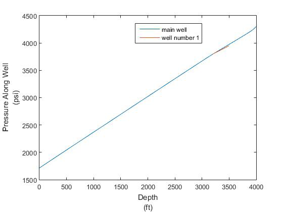
The results presented are derived from employing the reservoir and well properties explicated within this paper. Additionally, a notable detail is the establishment of the wellbore pressure for the lower formation, which is specified as 4300 psi (Figure 2).
The wellbore pressure associated with formation 1 is recorded as 3950 psi, indicating the pressure within the wellbore specifically pertaining to this formation. Additionally, the wellhead pressure, denoting the pressure at the wellhead, is documented as 1715 psi. These pressure values are crucial parameters in assessing the performance and dynamics of the production system (Figure 3).
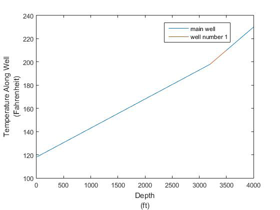
The specified temperature decrease is determined based on a geothermal gradient. From depths ranging between 3500 ft and 4000 ft, the temperature decreases at a rate of 2.5°F per foot. However, it’s noteworthy that there seems to be a discrepancy in the provided information, as it mentions both 2.5°F/ft and 2°F/ft for the same depth range. If we consider 2.5°F/ft as the correct value for this range, then the temperature decrease would be uniformly applied throughout. Clarification on the intended gradient for depths between 3500 ft and 4000 ft would be required to accurately interpret this information (Figure 4).
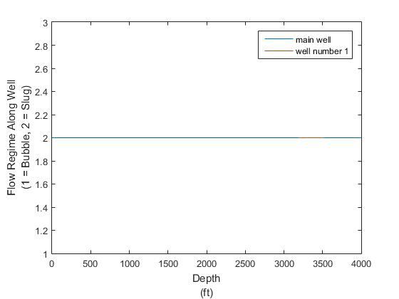
In this specific production system, the flow regime is identified as slug flow occurring throughout the well. Slug flow is characterized by the intermittent movement of liquid slugs separated by gas pockets within the flow stream. Understanding the flow regime is crucial for predicting and optimizing the system’s performance and behaviour (Figure 5).
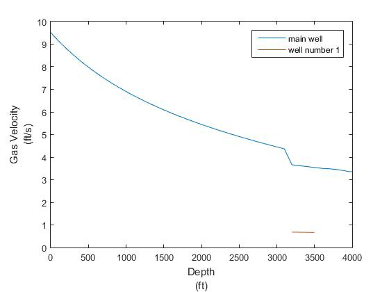
The gas velocity distribution along the well indicates variations in gas flow velocity at different depths. A notable feature in this distribution is a step increase, which occurs at a depth of 3200 ft. This increase in gas velocity is attributed to the introduction of gas flow from formation 1 at that specific depth. Understanding the distribution of gas velocity is essential for analyzing the flow dynamics and optimizing production operations within the well (Figure 6).
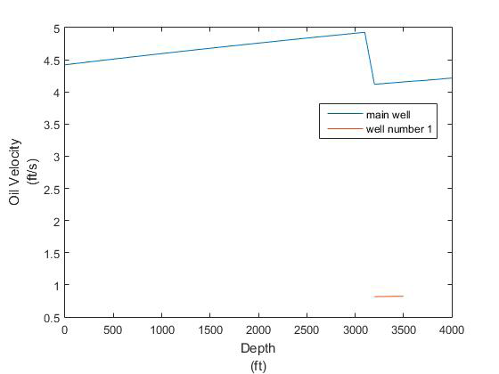
The oil velocity distribution along the well signifies the changes in oil flow velocity at various depths. Notably, a step increase is observed, specifically at a depth of 3200 ft. This sudden rise in oil velocity is directly associated with the introduction of oil flow from formation 1 at the mentioned depth. Understanding the distribution of oil velocity is vital for assessing the fluid dynamics and optimizing production strategies within the well (Figure 7).
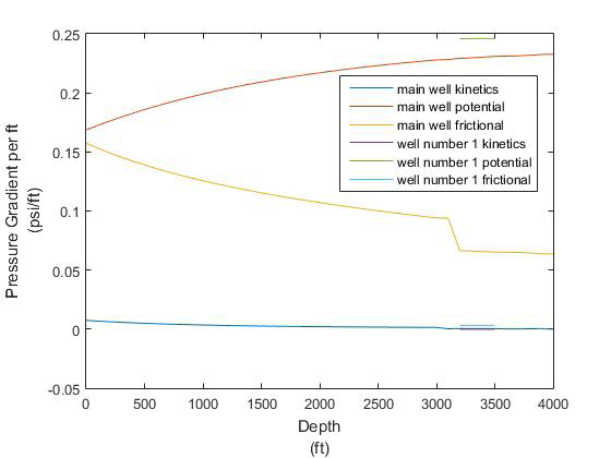
The figures provided depict the contributions of potential, kinetic, and friction pressure losses within the system. Notably, the analysis reveals that the predominant contributor to delta pressure per unit well length is the potential pressure drop. Following this, frictional pressure drop emerges as the second-largest contributor. However, the contribution from kinetic pressure drop is observed to be minimal, approaching zero across various points within the well. This finding corroborates the earlier assumption that the kinetic pressure drop can be considered negligible for the purposes of this analysis. Understanding these pressure contributions is essential for accurately assessing the system’s performance and optimizing its operational parameters (Figure 8).
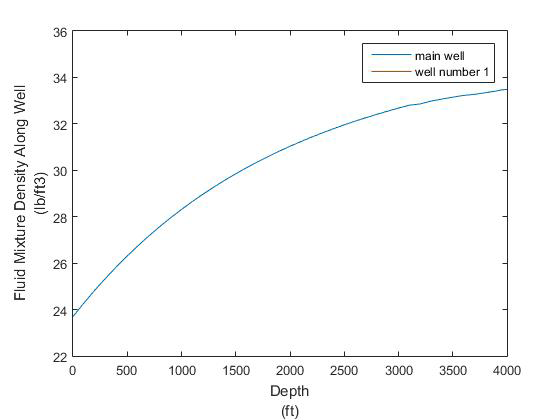
The observation made indicates that the mixture density diminishes as the fluid approaches conditions near the wellhead. This decline in density likely stems from changes in pressure, temperature, and the behavior of the fluid as it ascends towards the wellhead. Understanding this density variation is crucial for comprehending the fluid dynamics within the production system and optimizing operational strategies accordingly (Figure 9).
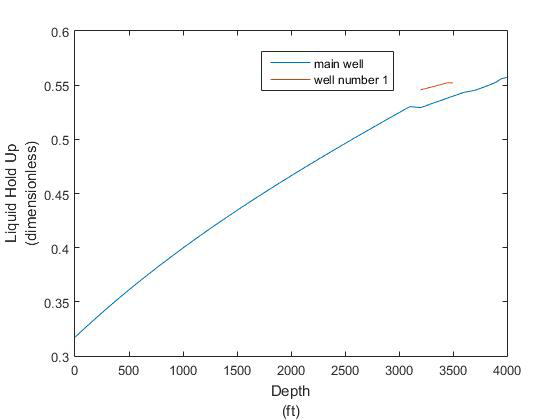
The trend observed suggests that the liquid holdup decreases along the length of the well, with a corresponding increase in the gas fraction as the well approaches the wellhead. This phenomenon likely arises due to the separation of gas and liquid phases as they ascend through the well, with gas accumulating towards the upper sections. Understanding this variation in liquid holdup is vital for predicting flow patterns and optimizing production strategies within the well. The simulator determines the gas production rate as 7479 barrels per day and the oil production rate as 3326 barrels per day. These volumetric flow rates are specified to be at wellhead conditions characterized by a temperature of 115 Fahrenheit and a pressure of 1715 psia. Understanding these production rates and their associated conditions is crucial for evaluating the performance of the production system and estimating resource yields accurately (Figure 10- 15).
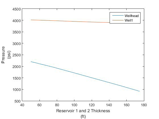
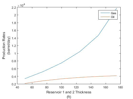
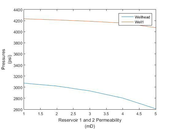
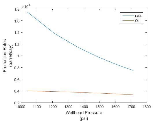
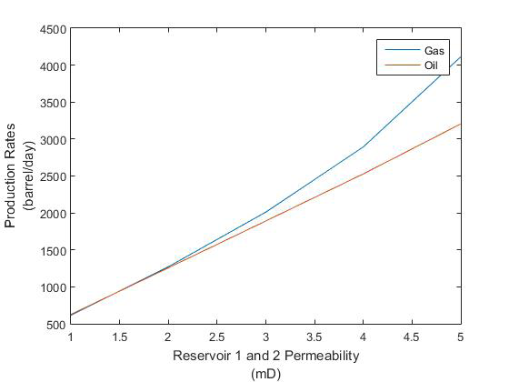
Figure 15: Varying Reservoir Permeability vs Constant Wellbore 2 Drawdown. In this study, we have endeavored to develop a comprehensive numerical simulator tailored for multilateral oil well systems, aimed at enhancing our understanding of their intricate dynamics and optimizing production strategies. Drawing upon established models such as Orkiszewski’s and Vogel’s, we constructed a versatile simulator capable of identifying flow regimes, calculating key parameters, and estimating production rates with precision. Through a series of simulations and analyses, we have illuminated the complexities inherent in multilateral oil well operations, shedding light on the interplay between reservoir properties, well geometry, and production performance. By leveraging physical assumptions and empirical models, we have crafted a pragmatic tool for reservoir engineers, offering valuable insights into system behavior and guiding decision-making processes. Our study has underscored the significance of key factors such as pressure behavior, fluid density variations, and flow regime transitions in shaping the performance of multilateral oil well systems. By elucidating these factors and their implications, we provide a foundation for optimizing production strategies, maximizing recovery rates, and mitigating operational challenges in real-world scenarios.
Looking ahead, further research endeavors may focus on refining the simulator’s predictive capabilities, integrating additional complexities such as non-Darcy flow effects or reservoir heterogeneities. Additionally, experimental validation and field-scale application of the simulator could offer valuable insights into its real-world efficacy and pave the way for practical implementation in industry settings. In conclusion, our study represents a significant step forward in the quest to unravel the complexities of multilateral oil well systems. By combining theoretical insights with practical simulations, we aim to empower reservoir engineers with the tools and knowledge necessary to navigate the challenges and opportunities inherent in modern oil production operations.
References
-
Orkiszewski J, Vogel JV (1986) Flow rate estimation in heterogeneous reservoirs. SPE Production Engineering 1(2): 155-160.
-
Lin B, Wei Y, Gao S, Ye L, Liu H, et al. (2024) Current Progress and Development Trend of Gas Injection to Enhance Gas Recovery in Gas Reservoirs. Energies 17(7): 1595.
-
Al-Kabbawi FAA (2024) The optimal semi-analytical modeling for the infinite-conductivity horizontal well performance under rectangular bounded reservoir based on a new instantaneous source function. Petroleum 10(1): 68-84.
-
Dundar EC, Alhemdi A, Gu M (2019) Impact of natural fracture-induced elastic anisotropy on completion and Frac design in different shale reservoirs. SPE/AAPG/ SEG Unconventional Resources Technology Conference, Denver, Colorado, USA.
-
Alagoz E, Giozza GG (2023) Calculation of Bottomhole Pressure in Two-Phase Wells Using Beggs and Brill Method: Sensitivity Analysis. International Journal of Earth Sciences Knowledge and Applications 5(3): 333-337.
-
Alagoz E, Mengen AE, Bensenouci F, Dundar EC (2023) Computational Tool for Wellbore Stability Analysis and Mud Weight Optimization v1.0. International Journal of Current Research Science Engineering Technology 7(1): 1-5.
-
Amin, Rana S, Abdulwahab, Ibrahim M, Rahman NMM (2024) Maximization of the Productivity Index Through Geometrical Optimization of Multi-Lateral Wells in Heterogeneous Reservoir System. International Petroleum Technology Conference, Dhahran, Saudi Arabia.
-
Alagoz E, Dundar EC (2023) A Comparative Analysis of Production Forecast for Vertical Gas Wells: Fractured vs. Non-Fractured. International Journal of Earth Sciences Knowledge and Applications 5(3): 333-337.
-
Aranguren, Cristhian, Araque R, Carlos, Cuervo, et al. (2023) Reducing Simulation Time in a Huff-And-Puff Gas Injection Project in Complex Shale Reservoirs: Sequence- Based Proxy Multi-Porosity Reservoir Simulator. SPE Canadian Energy Technology Conference and Exhibition, Calgary, Alberta, Canada.
-
Liu W, Zhao H, Sheng G, Andy LiH, Xu L, et al. (2021) A rapid waterflooding optimization method based on INSIM-FPT data-driven model and its application to three-dimensional reservoirs. Fuel 292(2021): 120219.
-
Alagoz E, Dundar EC (2021) A Comparative Analysis of Production Forecast for Vertical Gas Wells: Fractured vs. Non-Fractured. Journal of Petroleum & Chemical Engineering (JPCE), URF Publishers.
-
Alagoz E, Dundar EC (2024) Forecasting Gas Well Production and Analyzing Pressure Dynamics: A Study of Transient Flow and Pressure Drop in Natural Gas Formation. Journal of Energy & Environmental Science 2(1): 1-7.
-
Laalam A, Khalifa H, Ouadi H, Benabid MK, Tomomewo OS, et al. (2024) Evaluation of empirical correlations and time series models for the prediction and forecast of unconventional wells production in Wolfcamp A formation. SPE/AAPG/SEG Unconventional Resources Technology Conference, Houston, Texas, USA.
-
Dehdouh A, Bettir N, Khalifa H, Kareb A, Al Krmagi M (2024) Optimizing Recovery in Unconventional Reservoirs by Advancing Fishbone Drilling Technology in the Bakken Formation, Williston Basin. 58th U.S. Rock Mechanics/Geomechanics Symposium, Golden, Colorado, USA.
-
Vazquez M, Beggs HD (1980) Correlations for fluid physical property prediction. Journal of Petroleum Technology 32(6): 968-970.
-
Brill JP, Beggs HD (1972) Two phase flow in pipes. Proceedings of the 5th Annual North American Meeting, Society of Petroleum Engineers of AIME.
-
Lee JI, Gonzalez MH, Eakin BE (1982) A mechanistic model for two-phase flow in wells. SPE Production Engineering 3(4): 495-502.
- Nigeria’s Vulnerability in the Face of Global Energy Policy
- A Simulation Study of Investigation of Optimum Oil Production Performance by Applying Various Gas Injection Methods in Oil Reservoir
- Characterization of Permo-Triassic Reservoirs through Thermal Maturity Assessment of Westphalian Source Rocks in the Cheshire Basin
- Influence of Microwax on the Rheological and Thermal Behaviour of a Wax Crude Oil
- Real-Time Monitoring and Performance Optimization of Steam Injection in Heavy Oil Reservoirs Using Fiber Optic Sensing and Integrated Predictive Simulation Models
- Rapid On-Site Determination of the Total Petroleum Hydrocarbon Content of Soils by Handheld Fourier Transform Near-Infrared Spectroscopy: Development of a Global, Site- and Scanner- Independent Calibration Model