A Solid Body Model for Swirl Flow in Cylindrical Ducts

Background

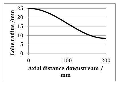
Lobate swirl-inducing ducts first appeared in a patent by a respected naval architect, E.F.Spanner [1, 2], who applied a helically-lobed tube for use in ships boilers to facilitate the efficient presentation of water for heat transfer. Raylor [3] proposed that the design should be applied to the transmission of difficult liquids, for example those bearing particles. When applied to this task the original 3-lobe design was found to be less efficient than 4-lobe or 2-lobe variants. An early fixed- pitch 4-lobe duct for particle bearing liquids is Illustrated in Figure 1. Later, this design incorporated a sigmoidal entry transition from circular to lobed profile (Figure 2), a fixed pitch central duct and a sigmoidal exit transition. This eliminated the practice of simply abutting cylindrical pipes at the entry and exit plane of a swirl duct causing attendant pressure losses. However the fixed pitch central section tended to constrain the angular acceleration of the transported media. Raylor [3] proposed a continually increasing spatial frequency to maintain the angular momentum of the duct contents. Current designs adopt this principle.

Click to enlarge

Click to enlarge

Since the early 4-lobe design, progress has been made in ducts with continually varying pitch and lobate form. The swirl is measured by a quotient known as the swirl number, Ω(also known as "swirl intensity")This is the ratio of angular momentum to axial momentum, non- dimensionalised with the duct radius, defined as follows R R uwr dr uwr dr

2 2 2 πρ ∫ ∫ Ω= =

0 0 2 2 2 (1)

R R RX u rdr R u rdr πρ

∫ ∫

0 0 Where R = pipe bore radius (of the cylindrical delivery pipe), u = axial velocity at radius r, 𝜌= fluid density and w = circumferential velocity at radius r. Another way in which swirl might be measured is the Swirl Angle,θ:

u θ − =      

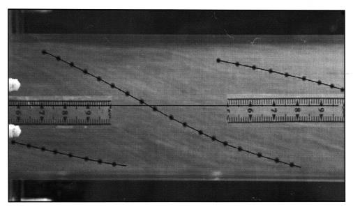
1 tan w Swirl angle is roughly proportional to swirl number for the solid-body model as will be demonstrated later. Swirl angle can be fairly easily estimated from transparent tube sections as shown in Figure 3.

Click to enlarge

This is a useful method when the calculation of swirl number using equation (1) is not possible.

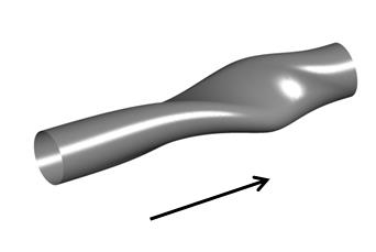
Figure 4 illustrates a 2-lobe, 180° tube with progressive pitch and a throat at a 2:1 position downstream to maximize the rotation given to the fluid. This is a low-loss design which was analysed with CFX software (Reynolds Stress Omega Model [4]). The model yields a pressure drop, ΔP, of 333 Pa over 0.3m. The swirl number was a modest 0.07 with swirl effectiveness_, Δ Ω = . For improved swirl numbers, current _p / 0.24 1 2 2 u ρ designs incorporate a twist slightly greater than a full 360° (actually 411°) to significantly improve the swirl number and to account for the lag of the transported medium.

Click to enlarge

Solid Body Model

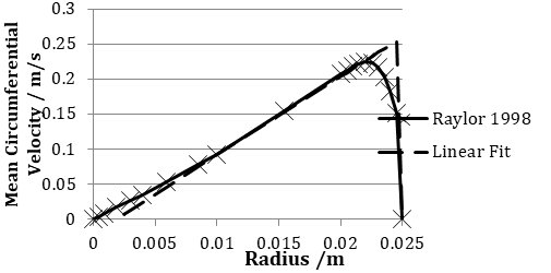
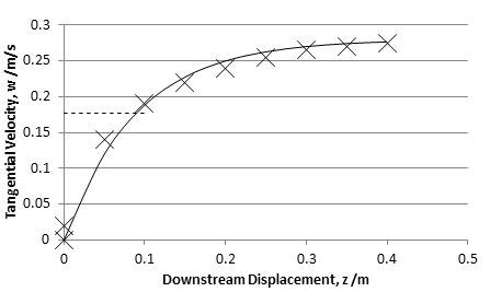
Figure 5 shows a tangential velocity profile for a nominal axial velocity of 2 m/s following a swirl duct. The near-linearity over approximately 84% of the bore indicates that angular velocity 𝜔, is almost constant in this range. Constant angular velocity is a characteristic of a solid rotating shaft and this concept suggests a simple mechanical analogy: The Solid Body Model. The data in this figure will be used to illustrate the model.

Click to enlarge

The swirl number quotient (equation (1)) can be considerably simplified if the tangential velocity w is replaced with ωr, whereω, the angular velocity over the linear region  is assumed to be constant.

1 tan 2 2 wR u θ Ω≈ ≈ (3)

Note that equation (3) indicates an approximately linear relation between swirl number and swirl angle for small values of w/u. This is important because ISO 5167 [5] and Halsey [6] characterize swirl in terms of swirl angle θ, rather than swirl number (Steenbergen [7]). Strictly, the graph in Figure 5 showed some departure from a linear law. Near the centre, the angular frequency was slightly less than the solid-body value, probably because the swirl had been created by a profile at the pipe wall. The peripheral 16% of the velocity profile indicates gathering damping friction as the radius increases. At the outer radial extremity, the circumferential velocity falls to zero in accordance with the no-slip principle of Newtonian mechanics. The swirl numberΩtakes account of these regions while the swirl angle, θ does not.

The expression for the torque of a rotating solid shaft is given by

2 θ θ θ θ = + + − (4)

( ) 2 d d M J c k o dt dt

where M is the torque on the notional solid shaft, J is the polar moment of inertia, c is the coefficient of damping and k is the stiffness of the shaft.

By definition liquids do not have stiffness, they adapt to the shape of their containment, so …

2 θ θ = + (5)

2 d d M J c dt dt

This expression has conveniently reduced to a first- order system in twist gradient dθ/dt with time constant given by J T C = (6) Convenient it may be, but equation (5) gives us the problem of defining a time-varying function for the torque input () before it can be solved. The dynamical system becomes much clearer when equation (5) is rewritten so that the dependent variable becomes axial distance along the cylinder (z). Putting G = twist gradient dθ/_dz and dividing throughout by _cu 𝑀 𝐽𝑢 𝑑𝐺 𝑑𝑧+ 𝐺 (7) Note that the group of variables at the left-hand side of equation [3] 𝐺𝐷(𝑧) = 𝑐𝑢= 𝐺𝐷(𝑧) = 𝑐 𝑀 𝑐𝑢 has the same dimensions as G and is the driving function, (torque per damping coefficient per axial velocity) i.e.

𝑑𝐺 𝑑𝑧+ 𝐺= 𝐺𝐷(𝑧) (8)

𝑇𝑢

Now the dynamics of the system is described by the properties of the profiled tube, particularly the swirl gradient dθ_/_dz inducing the swirl.

This time constant can be easily obtained from the polar moment per length J/L and the damping coefficient per length c/L.

𝐽

1

4 (9) 𝐿=

2 𝜌𝜋𝑅𝑦 where Ry is the radius of the rotating body. Referring to the example in Figure 4, the rotating solid body has a radius of 20.5mm in a duct radius of 25mm. Between this radius and the law of the wall we have a narrow motivating annular space in which the viscous damping and swirl decay take place. For a Newtonian liquid

2𝜋𝑅𝑦2(𝑅𝑦−𝛿) 𝑐 𝛿 (10) 𝐿= 𝜇 𝑅𝑦2𝛿

𝐽𝐿 ⁄

𝜌 Hence 𝑇=

(𝑅𝑦−𝛿) (11) 𝑐𝐿 ⁄ =

4𝜇 The time constant is strongly dependent on the bore of the duct, inversely dependent on the viscosity of the medium, but most importantly the radial width of the motivating annulus, δ. To help with the task of determining this width there are semi-empirical estimates of the time constant, T, for horizontal cylindrical ducts from Steenbergen [7] and Halsey [6] which allow equation (11) to be solved for δ.

ISO 5167 [5] specifies a 2° swirl-angle limit for measurement purposes and Steenbergen [7] came up with an empirical law, crucially including a friction factor (f ) to account for the natural roughness of the pipe bore, as follows Ω0 = 𝑒−𝜉𝑓𝑧 Ω(𝑧) 𝐷 (12) where Ω0 is the initial swirl number at the entry to the cylindrical duct.

There is a some uncertainty in the constant ξ and Steenbergen [7] suggests 𝜉= 1.49 ± 0.07. Much of the uncertainty is eliminated by factoring the friction factor in equation (12). A later study (Jones [8] has shown a value of 1.7 for perfectly smooth pipe wall, impossible to achieve in practice. When factored with a realistic friction factor (0.228), the value 𝜉= 1.483 is obtained. Making the assumption that the swirl angle is comparatively small, and 𝑡𝑎𝑛𝜃→𝜃 in equation (3), the swirl number can be substituted for swirl angle θ to give Halsey’s earlier correlation.

𝜃(𝑧) = 𝜃𝑜𝑒−𝜉𝑓𝑧 𝐷 (13)

This agreement on the constant ξ from three separate researchers is a rare event indeed_. Differentiating equation (13) with respect to downstream distance z, we have 𝑑𝑧= 𝐺0𝑒−𝜉𝑓𝑧 𝑑𝜃 𝐷 (14) where 𝐺0 = −𝜃0 ( 𝜉𝑓 𝐷) , a negative constant initial twist gradient (_i.e. a decaying gradient).

Taking Steenbergen’s value of ξ, this implies a time constant of 𝐷

1.49𝑓𝑢 (15) 𝑇=

For 50mm bore duct, friction factor 0.0228 and mean axial velocity 2m/s we get a time constant of 1.46s ± 0.07s for the case of the cylindrical duct data given in Figure 4_._ From Figure 4 we can assert 𝑅𝑦= 0.0205 (0.0045m from the wall). Solving equation (11) with the Steenbergen/ Halsey estimate of the time constant, we obtain the width of the motivating ring.

𝛿= 0.00029 𝑚 (16) The outer perimeter of the motivation ring is distant 0.0045 −0.00029 = 0.0042𝑚 from the pipe wall. It is now important to establish the thickness of the so-called “Law of the Wall” because, in theory at least, the boundary layer might encroach on the motivation ring. The law defines a non-dimensional quantity known as y+, the dimensionless distance to the wall, defined 𝑦𝑈∗ 𝜈 where y = distance from the wall 𝜏𝑊 𝑈∗ = shear velocity (√ 𝜌 where 𝜏𝑊 is the shear stress at the wall), and ν = kinematic viscosity 𝜇 𝜌 In the immediate proximity to the wall ( 0 ≤𝑦+ ≤5 ) is a laminar sub-layer. By definition a laminar region can provide no torque to the medium in the duct. Beyond this layer is the buffer layer through which the turbulent flow develops. The outer limit of this layer is indistinct, but has generally been accepted to lie between 𝑦+ ≈25 and 𝑦+ ≈50, typically 35. For the example 50mm bore duct, this gives an extent between 0.0001m and 0.00015m. In light of these calculations, it is reasonable to discount the laminar sub-layer and the buffer layer as influences in the outer radius of the motivation ring. They do not encroach upon it.

0.0045 ≥𝑦≥0.0042 𝑚 (17) Further, the Seventh Power Law (Prandtl [9]) indicates that at a radius of 0.205m in the example, the axial velocity is in fully turbulent flow and close the pipe mean velocity.

1 7 𝑢= 2.53 (0.0045 = 1.98 𝑚/𝑠

0.025 ) where 2.53 m/s is the maximum axial velocity predicted by the law.

Driving Function for the Generation of Swirl in A Profiled Duct

In contrast to the case of decay of swirl in a cylindrical tube, a profiled tube with a constant spatial frequency generates swirl (Figure 6).

Click to enlarge

In a profiled duct with progressive pitch, if the rate of increase in swirl gradient is λ, we have 𝑇𝑢𝑑𝐺 𝑑𝑧+ 𝐺= 𝜆𝑧+ 𝐺0 For the duct illustrated in Figure 3 the swirl gradient starts at zero (Go=0)

This yields the response of the rotating fluid as follows 𝐺(𝑧) = 𝑑𝜃 𝑑𝑧= 𝜆𝑧−𝑇𝑢𝜆(1 −𝑒−𝑧 𝑇𝑢) The solid body is a wall jet (Steenbergen [6]), roughly akin to a concentric tube rather than a solid shaft, with a very much smaller value for J, the polar moment of inertia, in consequence. The time constant is considerably smaller for the generation case as shown by Figure 6. See Jones [8, 10] for discussion of this issue.

Conclusions

Swirling flow in a duct has been shown to mimic a solid body with a motivating ring at its outer extremity. The main difference between a rigid solid body and a rotating body of fluid is in the transmission of torque. In a rigid body torque is transmitted by the stiffness of the body. In a rotating body of fluid there is no stiffness and the walls of the duct provide the torque. When the walls are helically profiled, positive swirl is generated. When the walls are cylindrical and unprofiled, a decay function is transmitted to the medium.

The decay of swirling flow in a cylindrical duct can be represented as a first order dynamical system with a time constant given by J/c, the polar moment divided by the coefficient of damping. There is a small motivating ring which has relatively small dimensions and contains the damping function.

The time constant of the system can be determined from equations for J and c. The formula for the polar moment J for a cylinder is well known. Less well known is an equation to determine the coefficient of damping, c, in terms of the Newtonian viscosity of the medium. It is critically dependent on the position of the motivating annulus (about 4mm from the wall in a pipe of 50mm bore) and for this reason is quite difficult to calculate. Fortunately, estimates of the time constant of the dynamical system for a cylindrical duct can also be made using semi-empirical correlations. The first of these to be used was developed by Halsey [6]. A later investigation by Steenbergen [7] confirmed his result. The width of the motivating annulus was estimated by equating these approaches with the value of the time constant described here.

The group Tu is a distance constant which comes from the dynamical equation (7). Since the system is a classical first-order system, it will reach 95% of its target after a downstream distance of 3_Tu_ metres. In the decay case this implies that 95% of the swirl will have dissipated after 3 × 1.46 × 2 = 8.76𝑚.

The first order system also applies to the generation of swirl in a profiled tube. In this case, the rotating body is a wall jet, of roughly cylindrical tubular form inside the profiled walls. The time constant for generation is significantly smaller than the time constant for decay (0.05s for the example). The swirl will have reached 95% of its target value after 0.3m. This dimension has been verified in tests and current designs for testing are 300mm in length.

References

-
Spanner EF (1940) British patent GB521548.
Spanner EF (1945) British patent GB569000.
Raylor B (1998) Pipe Design for Improved Particle Distribution and Improved Wear. University of Nottingham. **4.** ANSYS (2017) Omega Reynolds Stress model. ANSYS CFX-Solver Theory Guide, ANSYS Inc. Southpointe, Canonsburg, PA, pp: 95-96.
International Standards Organisation (2003) Measurement of Fluid Flow by means of pressure differential devices inserted in circular cross-section conduits running full – Part 1: General Principles and Requirements. 2nd (Edn.), Technical Committee ISO/TC30/SC 2 Pressure differential devices, pp: 33.
Halsey DM (1987) Flowmeters in Swirling Flows. J Physics E: Sci Instru 20(8).
Steenbergen W (1995) Turbulent pipe flow with swirl. TU Eindhoven.
Jones TF (2017) A Solid Body Model for Swirling Flows. 18th International Conference on Transport and Sedimentation of Solid Particles, Prague, Czech Republic,pp: 129-136.
Prandtl L (1921) Uber den Reibungswiderstand stromender Luft About the frictional resistance of strea ming air. Ergebnisse AVA Gottingen, pp: 136.
Jones TF (2019) Swirl-Inducing Ducts. _In:_ Boushaki T (Ed.), Swirling Flows and Flames. Intech Open.
- Sense, Gravity, Parity & Chirality in Mathematical Physics
- Quantum Lattice Simulations PHYSICS: Microcircuit Particle Formation and Observable Macroscopic Irreversible Time - A Discrete Lagrangian with Cellular Automata Framework
- Quantum Biology from Biomacromolecule to Cell, and Central Dogma Described by Quantum Theory
- Focus, Agility, Speed and Technology (FAST) for Sustainability and Growth
- Square Root Metric Geometry and Pati-Salam Model in Curved Space-Time
- A Simple System Demonstrating the Mpemba Effect in Classical Mechanics