Modeled Sea Level Rise Impacts on Coastal Vegetation and Infrastructure at Lake Earl Wildlife Area and Tolowa Lagoon, Northern California: Implications for Management and Adaptive Planning
Few ecosystems remain untouched by sea-level rise along the Pacific coast of North America. This process has facilitated reduction in the range of ecosystem responses and promoted loss of biological diversity at a scale relevant to local populations of plants and animals. Even fewer studies have evaluated the extent of rising sea levels on coastal ecosystems at finer scales. Here, I quantified the projected impacts of rising sea level on the vulnerability of plant communities at the Lake Earl-Tolowa Lagoon System (Lake Earl Wildlife Area) using a Static Vegetation Model. I also evaluated use of a recent regional coastal Marsh-migration Model fitted to the same study area. Results showed the Static Model predicted 100% of Estuarine Brackish Emergent habitat, 34.0% of Coastal Dune habitat, 80.7% of Freshwater Emergent Wetland, 48.9% of Forest Wetland, 21.0% of Grassland/Pasture, 8.0% of Coastal Maritime Forest, and 3.4% of Urban infrastructure would be inundated by salt-water at ~3.0m (~9.8 ft) of sea-level rise. Conversely, categories of marsh-types used in the Marsh-migration Model were inconsistent with the type of vegetation mapped within the study area, and impacts to these categories did not materialize until ~14 m (~45.9 ft) of sea-level rise. At this level Estuarian Wetland, Emergent Wetland, and Unconsolidated Shore exhibited slight increases in area, while other categories declined. The Marsh-migration Model also proved insufficient at identifying any major alteration in the extent of marsh-types for future planning or conservation by land managers, which was the primary goal of this model at conception. Identifying the potential impact of future sea-level rise on biological communities necessitates extensive data collection, quantification of plant and animal communities, updating existing vegetation maps, modeling the potential for migration inland, and establishing a comprehensive, multi-scale coastal-change modeling framework at spatiotemporal scales unique to the particular wildlife area. These actions are necessary to identify, assess, mitigate, and alleviate any potential future stressors in rising sea-level on natural resources on managed lands along the coast of northern California and elsewhere.
Abbreviations
CDFW: California Department of Fish and Wildlife; GIS: Geographic Information Systems; NOAA: National Oceanic and Atmospheric Administration; CRS: Coordinate Reference Systems; UTM: Universal Transverse Mercator; DEM: Digital Elevation Models; LiDAR: Light Detection and Ranging; WFO: Weather Forecast Office; MLLW: Mean Low Lower Water; MHHW: Mean High higher Water; LEWA: Lake Earl Wildlife Area
Introduction
Current estimates of the mean rate of rising global sea- level (gSLR) through the 21st century will cause fundamental ecological impacts across all coastal ecosystems, coincident with changes in storm frequency and intensity, and increased flooding and erosion. Adaptation to future sea-level rise and changing climate requires that resource managers on state and federal coastal lands understand the risk and vulnerability to their particular coastal ecosystem, such that management decisions are made at spatiotemporal scales relevant to maintaining biological diversity. Integrated monitoring and future planning will require focused and adaptive management actions that include future habitat changes within local coastal zones for the benefit of established ecological and social values.
Data gathered from satellite radar predicted an accelerating rise in gSLR of 7.5 cm from 1993 to 2017, which equates to an average rate of 31 mm per decade [1, 2]. If the forecast rate of increase in global temperature is limited to 1.5 °C, this would cause a gSLR between ~0.52 m (~1.7 ft) and ~1 m (~3.2 ft) by 2100 [3, 4, 5, 6]. This process will put many coastal ecosystems and the species that depend upon them at great risk. Global sea-level rise is primarily a function of thermal expansion of warming ocean water, infusion of fresh water from melting ice sheets and glaciers, and corresponding ocean expansion as seawater warms [6, 7, 8]. However, what is most important to maintaining coastal morphological equilibrium is not gSLR, but variance in the observed rate of relative sea-level rise (rSLR) at more local spatiotemporal scales of the coastline, coincident with the rate at which land elevation is changing [9, 10, 11]. This process will likely depart significantly from any predicted long-term gSLR [12, 13]. For instance, the rate of rSLR along the Pacific coast of North America is projected to increase from ~0.42 m (~1.4 ft) to ~1.7 m (~5.6 ft) by 2100 [14].
Estuaries and marshes within these tidal prisms perform invaluable ecosystem functions that shape biological communities at local scales [15]. Within these heterogeneous landscapes the rate of rSLR is driven by a multitude of covariate physical and climatic processes that vary in space and time [16, 17].
Salinization of coastal soils, wetlands, and upper reaches of estuaries and herbaceous wetlands cause intrusion of saltwater into surface and ground water. These processes function to raise water tables and impede drainage resulting in chronic losses of habitat [7, 16, 18]. Simultaneously, this process also reduces nutrient availability and absorption by resident vegetation, increases wave-height energy during storm surges and flooding at extreme high-tides, and inflates the rate of erosion [19]. Increases in deposition of suspended sediment within wetlands, above baseline levels and within upper reaches of estuaries, will force native plant communities to transition inland [20], causing beaches, dunes, and salt-brackish-freshwater marshes to migrate landward in response to rising sea level. If there is not available space, due to topography or established urban development, these systems will become part of the “coastal squeeze”, resulting in further loss, fragmentation, dispersion, or total loss of valuable resource space, ecosystem structure, and management infrastructure [21, 22, 23, 24].
Landscapes threatened by rising sea level may also experience tectonic processes of land movement at the local level. Uplift, deposition of sediments, and marsh accretion lessen the rate and amount of rSLR, while subsidence exacerbates and increases the amount of local upland land loss. Increased rates of sea water inundation may be particularly significant ecologically for obligate and endemic plant and wildlife marsh species [10, 25, 26], where loss of habitat, variance in water depth, and duration of saltwater saturation is crucial in structuring plant and wildlife communities [27]. Recent modeling predicts that changes in land elevation may degrade the overall habitat quality of salt marsh ecosystems, which are predicted to dominate in the latter half of the 21st Century as the rate of sea-level accelerates [25].
Areas that are particularly affected by rSLR include coastal lagoons systems, which may experience changes in circulation, tidal exchange during natural and anthropogenic breaching, turbidity, shrink in extent, re-connect with historically adjacent flood-plains and riverine systems, or disappear completely if blocked from migrating inland by agricultural lands and/or urban development [24, 28, 29, 30]. These process have the potential to dramatically affect the diversity of estuarian ecosystems and the species that occupy them. Yet relatively few studies have evaluated in detailed variance in the dynamics of coastal biological communities within these lagoon systems [11, 31, 32, 33, 34, 35, 36]. Navigating the challenge of coastal resource management over the ensuing decades therefore relies heavily on identification, quantification, modeling, and mitigation of the ecological consequences of rSLR at the local level (Figure 1).
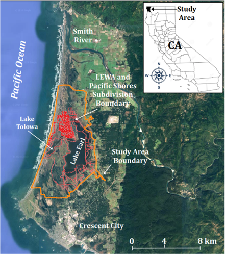
Here, I provide an example of how accelerated rates of predicted future sea-level rise may affect the extent and distribution of established vegetation communities on a state-owned wildlife area along the coast of northern California, with specific focus on a coastal lake-lagoon system and state managed wildlife area. My study focused on the area of mapped vegetation that currently surrounds and contains the Lake Earl Wildlife Area (LEWA) and Lake Tolowa Lagoon system (Figure 1; CDFW, 2003a). I used a Static Vegetation Model (constant in time) to quantify and evaluate the potential for future rSLR to adversely impact the extent and retention of mapped coastal vegetation vulnerable to flooding by saltwater intrusion [37, 38]. I also applied and evaluated the applicability of a recent regional Marsh-migration Model to the study area specifically. My study is timely and provides coastal resource managers additional knowledge necessary to anticipate, evaluate, and plan for the potential loss and mitigation of habitat and biological diversity against future rise in sea-level, which will negatively affect the ecology, recreational, and flood- protection services that this lake-lagoon system, and wildlife refuge provides [24, 39].
Study Area
The California Department of Fish and Wildlife (CDFW) LEWA encompasses Lake Earl, Lake Tolowa, and its companion lagoon system. The western edge of the area and refuge (~2,468.8 ha [6,100 ac]) borders the Pacific Ocean. Although called “lakes,” the Lake Earl/Tolowa complex is actually an estuarine lagoon. Acquired in 1975, LEWA was designated a priority acquisition by CDFW, which identified it as one of California’s 19th most productive wetlands. LEWA is located ~7.5 km (~4.7 mi) north of Crescent City, Del Norte County, along the northern coast of California (latitude ~41.8° N, longitude ~124.2° W; elevation ~14 m [~45.9 ft]; Figure 1). The combined surface area of these two lakes is ~2,023 ha (4,998.9 ac) with a perimeter of ~96.6 km (60.0 mi).
This portion of the Smith River Plain or Crescent City platform (~14,164 ha [~34.6 ac]) consists of a relatively flat coastal terrace at the base of the Coast Range Mountains bordering the Pacific Ocean [40, 41]. The Pacific Shores Subdivision (~307.6 ha [~760 ac]), at the northwest boundary of LEWA, consists largely of sensitive dune and wetland habitat.
This area was subdivided in the 1960’s into approximately half-acre lots and sold to individual lot owners. Because of the sensitive habitat, natural hazards, water quality concerns, and difficulty in siting development and infrastructure, such as sewage and water systems, it remains undeveloped and is slowly being acquired, lot-by-lot, by the State of California, Lands Program for incorporation into LEWA.
A coastal lagoon is defined as an “inland water body separated from the ocean by a barrier, connected to the ocean by one or more restricted inlets, which remain open at least intermittently, and has water depths that seldom exceed a few meters [34]. Within the LEWA there are two primary water bodies. The smaller body, closest to the ocean and the sandbar barrier beach is Lake Tolowa and its associated lagoon system. A large sandbar divides the lagoon from the Pacific Ocean, which breaches periodically, opening the lagoon to the sea. The larger body is Lake Earl proper. Lake Earl is primarily freshwater, and Lake Tolowa is moderately brackish. This lake-lagoon system consists of a mosaic of coastal habitat with a diverse array of flora and fauna, which include special-status plants and wildlife. Rainfall and surface lake elevation fluctuates seasonally to a great extent. Time series analyses found a significant decreasing trend in seasonal surface lake elevation but no trend in rainfall [41]. A declining trend in surface elevation in combination with variation in the historical area and extent of wetland plant communities may be attributable to systematic breaching of the lagoon annually, which periodically interrupts the natural functioning of the lake-lagoon system.
The Lake Earl/Tolowa complex is the largest coastal lagoon system on the Pacific coast south of Alaska. This estuarine lagoon system and its tidal prism are fed by heavy winter rains, various streams within the coastal plain, and numerous sources of groundwater [40, 41]. Together these lakes constitute the largest lagoon system, and third-most important seabird area on the West Coast after the Farallon and the Channel islands in southern California [42]. The Lake Earl/Tolowa complex also lies within the Del Norte Coast Important Bird Area, and the Audubon Society has identified this area as one of the most ornithologically significant coastal bird areas in the State, with ~300 bird species documented [43].
Further, the Lake Earl/Tolowa complex provides habitat for ~14 federally listed species, ~40 species of California Species of Special Concern, ~21 species of fish, ~40 species of mammals, and > 500 species of species. During seasonal migrations the wetland complex hosts > 100,000 birds. Lakes Earl and Tolowa also play a significant role in regional recreation, flood control, and proper functioning of onsite wastewater systems, wells, and management of landscape- level runoff from storms and seasonal rains. Intrinsically, management of the LEWA and lake-lagoon complex constitutes a critical part of successful natural resource planning, monitoring, and mitigation of variance in future rSLR, as relates to the evolution of biological systems along the extreme northern coast of California.
Methods
Datasets
Availability of coastal satellite data and data assimilation techniques by use of Geographic Information Systems (GIS) provides an opportunity to evaluate rising sea-level processes at a local level [39]. All GIS vector and raster datasets used herein were obtained from the National Oceanic and Atmospheric Administration (NOAA) Coastal Services Center’s Digital Coast website [44]. A digital copy of mapped vegetation [42], surrounding and including the LEWA and Lake Earl/Tolowa complex, is available from the CDFW GIS office in Eureka, CA. Coordinate reference systems (CRS) for all data were re-projected to the Universal Transverse Mercator (UTM), NAD 83, Zone 10, and clipped and polygonized to the boundary of the existing study area vegetation map, which is the reference site for my investigation [45].
High-resolution digital elevation models (DEM) were a part of a series produced for the NOAA Coastal Services Center’s Sea Level Rise and Coastal Flooding Impacts Viewer [46]. DEMs were derived from the best available Light Detection and Ranging (LiDAR) data collected for the California Coastal Conservancy between 2009 – 2011. DEMs were developed using the NOAA National Weather Service’s Weather Forecast Office (WFO) boundaries. The WFO DEM was divided into smaller regional DEMs to ensure more manageable file sizes. The Eureka (CA) WFO DEM was split into two smaller DEMs divided along county lines that included Humboldt and Del Norte counties. These “regional” county-wide DEMs were mosaiced together and resampled to ~5 m (~16.4 ft) resolution.
Vegetation-Types
Coastal vegetation communities that surround the study area and Lake Earl/Tolowa complex exist within an established tidal elevation range, given the environmental tolerance of endemic vegetation-types and salinity impacts from inundation. Vegetation communities along the shoreline and inland non-aquatic vegetation (terrestrial coastal vegetation) are shaped by climate, historical changes in sea level, and variation in the supply of sediment to the coastline. The seven major vegetation-types mapped for the study area also constitute the primary plant communities for resident and migrating species of wildlife (Figure 2; Table 1) [42, 47, 48].
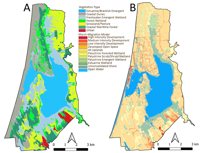
Figure 2: A) Map of the existing vegetation-types found within the study area and used in the Static Vegetation Model; and B) baseline (zero sea-level) map of various hypothetical numbered categories of marsh-types derived from the Marsh Migration Model, based on a clipped and vectorized digital elevation model (DEM) that used the NOAA National Weather Service’s Weather Forecast Office (WFO) boundaries.
| Primary Vegetation-type | Composition of Common Plant Species |
|---|---|
| Estuarian Brackish Emergent | Open water, flooded and non-flooded mud/sand-flats vegetated by sago pond weed (Potamogeton pectinatus), widgeon-grass (Ruppia maritima), stonewort, and seashore salt- grass (Distichlis spicata) |
| Coastal Dunes | Bare sandy shoreline and sparsely vegetated with scattered European beach-grass (Ammophila arenaria), sand verbena (Abronia latifolia), beach buckwheat (Eriogonum latifolium), beach sagewort (Artemisia pycnocephala), silver bursage (Ambrosia chamissonis), beach evening primrose (Camissonia cheiranthifolia), silvery phacelia (Phacelia argentea), early blue violet (Viola adunca), and a variety of grasses and forbs. Blue violets are the primary larval host plant for the federally listed Oregon silver spot butterfly (Speyena zerene hipployta). |
| Freshwater Emergent Wetland | Broad-leaf cattail (Typha latifolia), giant burreed (Sparganium eurycarpum), marsh cinquefoil (Potentilla palustris), mare’s-tail (Hippuris vulgaris), floating pennywort (Hydrocotyle ranunculoides), slough sedge (Carex obnupta), water parsley (Oenanthe sarmentosa), watercress (Nasturtium officinale), spikerush (Eleocharis macrostachya), Pacific silverweed (Potentilla anserina), tufted hairgrass (Deschamsia caespitosa), reed canary grass (Phalaris arundinacea), various rushes (Juncus sp.), and creeping buttercup (Ranunculus repens). |
| Forest Wetland | Willows (Salix hookeriana, S. sitchensis, S. laseolepis), red alder (Alnus rubra), Sitka pruce (Picea sitchensis), skunk cabbage (Lysichiton americanum), thimbleberry (Rubus parviflorus), Oregon crabapple (Malus fusca), and twinberry (Lonicera involverata). |
| Grassland/Pasture | Flooded and non-flooded areas of velvet grass (Holcus lanatus), sweet vernal grass (Anthoxanthum odoratum), orchard grass (Dactylis glomerata), tall fescue (Festuca arundinacea), soft chess (Bromus hordeaceus), barley (Hordeum sp.), sheep sorrel (Rumex acetosella), English plantain (Plantago lanceolata), iris (Iris douglasiana), European beach grass, and lupine (Lupinus bicolor). |
| Coastal Maritime Forest | Predomanitly upland forest of Sitka spruce (Picea sitchensis), grand fir (Abies grandis), beach or shore pine (Pinus contorta ssp. Contorta), and introduced Monterey cypress (Cupressus macrocarpus); understory species of twinberry, hairy honeysuckle (Lonicera hispidula), dogwood (Cornus stolonifera), silk tassel (Garrya elliptical), salal (Gaultheria shallon), Pacific wax myrtle (Myrica californica), Oregon crabapple, and cascara (Rhamnus purshiana); scrub and deciduous hardwood species of red alder (Alnus rubra), willow (Salix sp.), and red- berried elder (Sambucus racemosa). |
| Urban | Urban development consists of a small component at the extreme southwestern end of the study area. |
Table 1: Plant community types and associated species of plants contained within these primary vegetation-types mapped within the
Relative Sea Level Rise
Variability in rising and sinking of land across the ~1350-km-long (839 mi) coast of California was recently highlighted in a detailed (~100-m [~328.1 ft] resolution) and high precision (~1 mm/year [0.04 in]) map provided by the National Aeronautics and Space Administration (NASA) [12], Earth Observatory; and for coastal northernmost California [12, 16, 49]. At a regional level, measurements derived from variance in sea-level, highway level surveys, and Global Navigation Satellite System data concur that land is rising at Crescent City (~11.7 km [~7.3 mi]) south of the study are and LEWA, but it is subsiding in Humboldt Bay, ~193.1 km (~120 mi) south of LEWA [49]. By subtracting absolute sea- level rates from measurement gauges at Crescent City versus Humboldt Bay (~135.2 km [~84 mi] apart), the hypothesized relative rate of uplifting at Crescent City was estimated to be ~2.83 mm/year (~11.1 in) versus a subsidence rate of ~3.21 mm/year [~0.13 in] for Humboldt Bay [49]. Assuming that the rate of uplifting within the study area and LEWA mirrors that of Crescent City, it is possible to assess the potential influence of rSLR at a local level in relation to the existing plant communities within the study area. A detailed analysis of sea-level rise vulnerability assessment for California state wildlife areas surrounding Humboldt Bay, Humboldt County, northern California is also provided elsewhere [24].
Sea level rise digital files were clipped to the study area vegetation map and polygonized to describe the area potentially inundated by rising sea-levels across the landscape [45]. I used a Static Vegetation Model as a first step in assessing the overall potential for rSLR to affect change in the existing plant-associated landscape structure. This model assumed that: 1) inundation of water from rising sea- level would logically follow the contours of the landscape within the watershed; 2) sediment loads, freshwater input from the watershed, organic matter production, and rates of decomposition and compaction were constant through time; and that existing vegetation would be expected to get squeezed but not transition inland. Although this model does not account for up-slope migration of preexisting vegetation, it provides an initial first-step, from a logistic and cost-effective perspective, in assessment of plant community resiliency in response to rSLR.
Marsh Migration
I used the Marsh-migration Model developed by the NOAA Office for Coastal Management Marsh Migration to represent the hypothesized distribution of marsh-types based on elevation and frequency of inundation under the influence of future rise in sea-level [50]. This model assumes that as sea level rises: 1) higher elevations are increasingly inundated, allowing for hypothesized categories of marsh- types to migrate landward; 2) that some lower-lying areas will be inundated such that marshes will no longer be able to survive and be lost to open water; and 3) in some areas rising sea-levels may also cause accretion of inter-tidal sediments, where wetland vegetation can generate or capture sediments at rates exceeding rSLR [20, 51].
At the regional level, geospatial data layers were developed for coastal northern California (Humboldt, and Del Norte counties). A tidal zone raster was created for each increment of rising sea-level using a 10-m DEM of state and tidal surfaces created from NOAA’s vertical datum, representing shoreline data at Mean Low Lower Water (MLLW) and Mean High higher Water (MHHW). The tidal zone raster for each increment in rising sea-level (~0-3.1 m [~10 ft] in ~0.15 m [~0.5 ft]) was combined with a re-coded land cover raster to create a new raster, where pixels have both a tidal zone and a land cover code. Using a rule-set that says which land cover types exist in each tidal zone, the combined raster was re-coded to a new land cover raster where the land cover class changed based on the tidal zone [50]. The resulting hypothetical categories, and model-assigned numbers, within the modified land cover source data specific to the region where: 2 = High Intensity Developed, 3 = Medium Intensity Developed, 4 = Low Intensity Developed, 5 = Developed Open Space, 8 = All Uplands, 13 = Palustrine Forested Wetland, 14 = Palustrine Scrub/Shrub Wetland, 15 = Palustrine Emergent Wetland, 18 = Estuarine Wetland, 19 = Unconsolidated Shore, and 21 = Open Water.
This Marsh-migration Model provides an excellent opportunity to evaluate the applicability of this “regional” shoreline inundation model in anticipation of future rSLR. Although it is not a locally defined model specific to the study area, it provides a more realistic spatiotemporal alternative to models built from gSLR estimates. In adapting this model to my study area, I used the MHHW tidal datum in all analyses because I wanted to maximize the potential impact of rSLR on plant resources in anticipation of the worst-case scenario for threat assessment and future management purposes. I then clipped and polygonized the modified land cover layer (Marsh-migration Model) to the study area (vegetation map) [45]. Additionally, this regional county-wide Marsh- migration Model provides the foundation for the interactive geospatial map used in the “Lands Viewer” developed by CDFW for the entire coastline of California [52].
Results
Comparison of Vegetation-Types to Marsh-Types
As expected, various existing vegetation-types and predicted baseline (at sea-level) categories of marsh varied in their distributions throughout the study area (Figure
2). The most common plant-type communities consisted of Freshwater Emergent Wetland, Estuarian Brackish Emergent, and Grassland/Pasture (Figure 3A, Table 2); whereas the most common predicted marsh-types assigned by the baseline marsh-migration model, were All Uplands and Open Water categories (Figure 3B). A comparison of marsh- types, identified in the baseline Marsh-migration Model, clipped to the study area, with the current vegetation map showed that the All-Uplands category populated virtually all vegetation-types within the focal area (Figure 3C). The only exception being Estuarian Brackish Emergent habitat, which matched almost entirely the Open Water category of the marsh-migration model. Conversely, virtually all categories within the Marsh-migration Model were populated by nearly all of vegetation-types found within the study area (Figure 3D). Here the exceptions were again Estuarian Brackish Emergent versus Open Water, but also Coastal Dunes versus Unconsolidated Shore. Importantly, although the model of marsh-migration assigned areas of High, Medium, and Low (4) intensity development, there were no such categories within the study area. Therefore, I removed these marsh- migration assemblages from any further consideration.
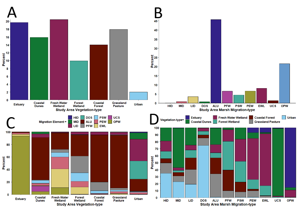
Figure 3: Bar graphs of the percent composition of A) current vegetation-types, B) categories of predicted marsh-migration habitat-types, C) vegetation-types that make up categories within the baseline Marsh-migration Model, and D) categories within the of baseline Marsh-migration Model found within the current vegetation-types. Colored bars are consistent throughout each comparison between vegetation- and marsh-types categories. HID = High Intensity Developed, MID = Medium Intensity Developed, LID = Low Intensity Developed, DOS = Developed Open Space, ALU = All Uplands, PFW = Palustrine Forested Wetland, PSW = Palustrine Scrub/Shrub Wetland, PEW = Palustrine Emergent Wetland, EWL = Estuarine Wetland, UCS = Unconsolidated Shore, and OPW = Open Water.
| Vegetation-type | Area | Perimeter | ||
|---|---|---|---|---|
| Hectares | percent | km | percent | |
| Coastal Dunes | 824.5 | 15.9 | 131,973.60 | 16.5 |
| Coastal Maritime Forest | 725 | 14 | 125,398.70 | 15.7 |
| Estuarian Brackish Emergent | 1,020.10 | 19.7 | 31,721.70 | 4 |
| Forest Wetland | 516.1 | 10 | 159,419.30 | 19.9 |
| Freshwater Emergent Wetland | 1,057.80 | 20.4 | 185,885.80 | 23.2 |
| Grassland/Pasture | 928.5 | 17.9 | 152,687.10 | 19.1 |
| Urban | 103.1 | 2 | 13,188.60 | 1.6 |
| Total | 5,175.10 | 100 | 800,274.80 | 100 |
| Categories of marsh-types in migration model | Area | Perimeter | ||
| Hectares | percent | km | percent | |
| High Intensity Development | 3.8 | 0.1 | 3,280.00 | 0.2 |
| Medium Intensity Development | 45.9 | 0.9 | 36,340.00 | 2.4 |
| Low Intensity Development | 186 | 3.6 | 160,580.00 | 10.7 |
| Developed Open Space | 40.1 | 0.8 | 25,580.00 | 1.7 |
| All Uplands | 2,364.40 | 45.8 | 470,960.00 | 31.5 |
| Palustrine Forest Wetland | 338.1 | 6.5 | 190,840.00 | 12.7 |
| Palustrine Scrub/Shrub/Hardwood Wetland | 233.1 | 4.5 | 149,340.00 | 10 |
| Palustrine Emergent wetland | 343.8 | 6.7 | 180,800.00 | 12.1 |
| Estuarine Wetland | 422.2 | 8.2 | 153,460.00 | 10.2 |
| Unconsolidated Shore | 74 | 1.4 | 43,920.00 | 2.9 |
| Open Water | 1,115.90 | 21.6 | 82,340.00 | 5.5 |
| Total | 5,167.40 | 100 | 1,497,440.00 | 100 |
Table 2: Baseline areas and perimeters of existing vegetation-types used in the Static Vegetation Model within the study area and
Table 2: Baseline areas and perimeters of existing vegetation-types used in the Static Vegetation Model within the study area and categories of marsh-types designated by the baseline (sea-level) Marsh Migration Model; km values represent summaries of the estimated perimeter distances of each fragmented vegetation-type (Static Vegetation Model) and marsh-type category (Marsh-migration Model).
Elevation of Vegetation-type and Marsh-types
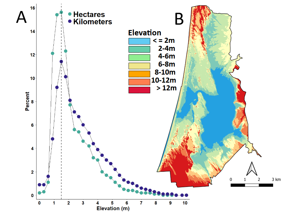
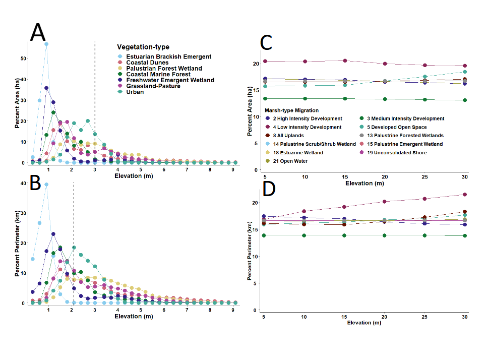
Elevation of the study area ranged from sea level to ~10.0 m (~32 ft; Figure 4A). The most common elevation was ~1.5 m (4.9 ft), after which the percent frequency of both area and perimeter decreased precipitously. Topography varied considerably across the landscape, with regions of highest elevation located at the extreme northern, southern, and eastern boundaries of the study area (Figure 4B). All plant communities were primarily restricted to locations between sea-level and ~ 3 m (~9.8 ft) in elevation. After ~5 m (~16.4 ft), all existing vegetation-types decreased progressively in percent area and perimeter out to ~9.0 m (~30.5 ft) of elevation (Figures 5A & 5B).
As for the baseline Marsh-migration Model, all categories of marsh plotted well beyond the elevational range and scale of existing plant communities within the study area (Figures 5C & 5D). Here, all categories of marsh were similar in area and perimeter of habitat from ~5m (~16.4 ft) out to ~30 m (~98.4 ft) in elevation. There was only a slight up- tick in the predicted area of Developed Open Space; and a slight down-tick in the predicted area of Unconsolidated Shoreline, which was accompanied by an increasing trend in the perimeter of this category beginning at ~5m (~16.4 ft). Perimeter estimates of all other categories of marsh retained a relatively flat trajectory.
Static Vegetation Model Versus Sea-level Rise
The Static Vegetation Model (Figure 6A) for current plant communities showed relatively little change in the total area of each vegetation-type until ~1.2 m (~3.9 ft) in rSLR) (Figures 6B & 6C). At ~3.0 m (9.8 ft), however, the model predicted 100% inundation of Estuarine/Brackish Emergent habitat, and a reduction in total area of Coastal Dune by 34.0%, Freshwater Emergent Wetland by 80.7%, Forest Wetland by 48.9%, Grassland /Pasture 21.0%, Coastal Maritime Forest 8.0%, and Urban infrastructure by 3.4% (Table 3). Except for Estuarine/Brackish Emergent habitat, the perimeter of all other patches of vegetation followed similar declining trajectories as their areas and perimeters. For Estuarine/Brackish Emergent habitat, after initially decreasing at ~1.2 m (3.9 ft) of inundation the perimeter of this habitat-type gradually increased beginning at ~1.5 m (4.9 ft) of rSLR, which was presumably a function of expansion, diversification, and increased fragmentation within a diverse inland landscape.
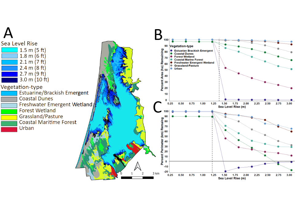
Figure 6: A) Map of the study area boundary showing the predicted levels of inundation by rising sea-level superimposed onto existing vegetation-types and the predicted B) decrease in area and C) perimeter of vegetation-types. The ~3 m rise in sea-level corresponds to that predicted by the year 2021, which assumes the forecast rate of increase in global temperature is limited to ~1.5 °C.
| rSLR Inundation | Community Vegetation-type | Infrastructure Affected by Rising Sea- level |
|---|---|---|
| ~0.3 – 1.2 m (~1 – 4 ft) | Coastal Dunes; Marine Forest | Loss of 3.7% total area and 11% of perimeter, and a loss of 1.9% of perimeter, respectively. |
| ~1.5 m (~5 ft) | Herbaceous and scrub wetland within the Coastal Dune layer. | Surrounding all parcels within the Pacific Shore Subdivision. |
| Isolation of numerous parcels between beach and Lake Tolowa. | ||
| Inundation of all LEWA boundaries with water levels reaching Kellogg Rd at its norther boundary | ||
| Begin flooding of suitable blue violet habitat | ||
| Inundation of Lower Lake Rd along entire eastern boundary of LEWA. | ||
| Lake Earl Road and Buzzini Rd along southeast corner edge. | ||
| Inundation of Old Mill Road at southern tip of LEWA boundary. | ||
| Inundation of Septic tanks begins in the north and south along Lake Earl Road, with most septic tanks fully inundated at ~3 m (~10 ft) along the LEWA side of the Study Area. | ||
| Virtually all CDFW facilities encroached or flooded. | ||
| ~1.8 m (~6 ft) | Herbaceous and scrub wetland within the Coastal Dune layer, and edges of Coastal Marine Forest. | Inundation and over-topped of Kellogg Rd and several locations along Lower Lake Rd |
| Beginning of encroachment into the edge of agricultural lands within the Grassland/Pasture layer. | ||
| ~2.1 m (~7 ft) | Herbaceous and scrub wetland within the Coastal Dune layer, and edges of Coastal Marine Forest. | Beginning of many of the edge parcels within the Pacific Shores Subdivision are flooded and flooding beginning at edge of County flood boundary. |
| Further encroachment into edge of agricultural lands within the Grassland/Pasture layer. | Kellogg Rd completely cut off from the beach . | |
| ~2.4 m (~8 ft) | Inundation of herbaceous wetland, scrub wetland, dune mat, and European beach grass within the Coastal Dune layer, and edges of Coastal Marine Forest layer. | Inundation reached paved edge of Lake Earl Dr. in several locations and inundation continues at County flood boundary. |
| Beginning of encroachment into the edge of agricultural lands within the Grassland/Pasture layer. | ||
| ~2.7 m (~9 ft) | Native-dominated meadow within Coastal Dune layer. | 50% of all parcels flooded within SW portion of subdivision. |
| Beginning of encroachment into edge of agricultural lands within the Grassland/Pasture layer. |
Table 3: Relative rise in sea-level (rSLR) and potential effects of anticipated inundation of saltwater into the study area and L
- Total flooding of CDFW headquarters, shops, barns, property of numerous local residents, particularly along the NE boundary of
- LEWA.
- Water bodies along Lake Earl Dr and > 60% of subdivision parcels flooded.
- Dune mat, open sand, European beach grass, within the
- Coastal Dune layer, scrub wetland, herbaceous wetland within Forest Wetland. Maximum encroachment into agricultural lands within Grassland/Pasture layer and edges of Urban habitat.
- Increased connection between lakes and lagoon.
- ~3.1 m (~10 ft)
- Flooding outskirts (~1,221 m [~0.7 mi]) of residential areas boarding northern edge of Crescent City and Smith River drainage
- (~2,103 m [~1.3 mi]).
- 83.3% (n = 18) of the wells on LEWA flooded.
Table 4: Relative rise in sea-level (rSLR) and potential effects of anticipated inundation of saltwater into the study area and Lake
Results also show impacts to the surrounding infrastructure at LEWA from inundation by seawater, which materialized at ~1.5 m (~4.9 ft); and by ~3.0 m (~10 ft) flooding inland continued in all directions (Figure 7).
This would include encroachment on residential outskirts boarding the northern edge of Crescent City and the main- stem of the Smith River, along an existing historical drainage to the north.
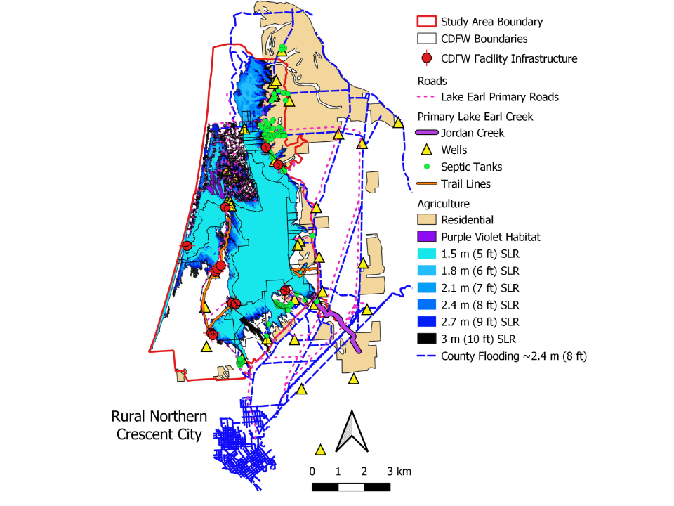
Such an extension would likely re-establish the original historical connection between the lake-lagoon system and the Smith River drainage (Figure 1) [53]. More importantly, in combination with high tides, storm surge, and flooding during the rainy seasons, rSLR at this level could cause: 1) an island-like effect on habitat separated by an expanded Lake Earl–Lake Tolowa system and the Smith River corridor, 2) a bay-like system as a function of expansion and coalescence of the original lake-lagoon system to the north and south, and/or 3) subsequent loss of a dynamic functioning lagoon ecosystem.
Marsh-migration Model Versus Sea Level Rise
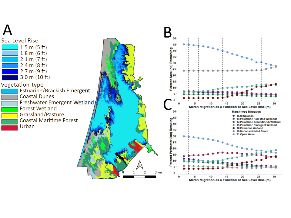
For comparison with vegetation-types, the map in Figure 8A shows the pattern of rising sea-level superimposed onto the baseline Marsh-migration Model [50]. In contrast, Figures 8B & 8C illustrate future predictions of the Marsh- migration Model for areas and perimeters of each theoretical category of marsh.
Compared to the Static Vegetation model, the Marsh- migration Model transitioned out to 30 m to much higher elevational levels into the upper watershed, which were well beyond the range of the current vegetation map. Importantly, potential impacts of rising sea-level on areas and perimeters of marsh-type categories did not materialize until ~14 m (45.9 ft) of rSLR inundation. At that level, Estuarian and Palustrine Emergent wetlands slowly increased in both area and parameter, while all others categories slowly declined. Open Water, Palustrine Forest Wetland, and Unconsolidated Shore exhibited a slow decline early on beginning at ~2.5 m (8.2 ft). These trends in regional marsh-migration continued throughout the projection of the model for each marsh-type category.
Discussion
Climate change-induced rising sea-level poses a severe threat to the establishment and maintenance of biological diversity in coastal-marine and near-shore terrestrial ecosystems. This process is largely the result of the accelerated magnitude and spatiotemporal extent of weather-related storm surge (high and King tides) on immensely complex shorelines, estuarine embayment, and lagoon systems found within low-lying, tidally-influenced seascapes [11, 54, 55].
Based on recent modeling, coastal wetland ecosystems will be substantially impacted, irrespective of variance in future predicted rates of gSLR [1, 4, 9, 10, 56, 57, 58]. As a consequence, critical challenges to coastal land managers responsible for conservation of natural resources on state and federal properties in the foreseeable future, which include: 1) evaluating the impact of rSLR on coastal lagoons and estuaries, 2) assessing how rSLR will manifest at different spatiotemporal scales, and 3) how effects of rSLR can be monitored and mitigated in a comprehensive and integrated way.
As a preliminary first step, and without knowledge of plant community migration inland, predictions of the Static Vegetation Model showed that rSLR will impose significant changes in extent of existing plant communities within the study area. Reduction in area and fragmentation of vegetation will also significantly and adversely impact endemic and obligatory plant and wildlife species, including those currently under state and federal protection. For instance, recent research that combined long-term data collection with modeling of: 1) rSLR, 2) coastal geomorphology, 3) adaptive behavior of species, and 4) population dynamics of shorebird populations showed that habitat quality declined rapidly owing to nest flooding, such that that populations were projected to collapse well before their species-specific habitat was totally inundated [59]. These authors hypothesized that focusing only on habitat loss underestimates impacts to biodiversity from sea-level rise, and that populations of shorebirds will suffer sooner than predicted, despite adaptively migrating to higher grounds. Their results and conclusions likely also apply to most wildlife species that occupy the interface between the coastal tidal prism and adjacent terrestrial upland ecosystems as reflected in numerous other studies [33, 60, 61, 62, 63, 64].
Importantly, there is also the need to empirically evaluate the potential for variance in the succession of plant community structure and distribution within the study area based on other environmental covariants. Elsewhere, I showed that the process of “natural” succession in the evolution of vegetation-types within the study area was relatively minor between 2002 to 2014 [41]. For this period, only ~2.1% (106.5/5,175.1 ha) of the total vegetated area appeared altered within the study area, which likely also included rSLR to some degree. Yet to what degree variance in plant communities and dependent wildlife species will be affected by other covariant drivers remains to be determined through empirically-driven monitoring and integrated modeling. Such drivers may potentially include variance in muted subsidence, sediment delivery from the watershed transported via several streams, infusion of sand from the ocean side of the tidal prism of the lagoon, plant productivity, erosion, factors associated with climate change (temperature and precipitation; Sullivan, 2002) and its effects on plant productivity, availability of up-slope migration, and adjacent land-use practices [9, 65].
Although coastal habitats to some extent may be able to accommodate moderate changes in rising sea-level by continuous migration inland, the opportunity for inland migration along much of coastal northern California has been reduced considerably given the accelerating pace of sea-level rise [24]. In my study the only projected expansion was associated with Estuarine/Brackish Emergent habitat (open water, flooded and non-flooded mud/sand-flats, etc.). Future expansion of this habitat-type inland, following rSLR, will encroach eastward into the adjacent agricultural and urbanized landscape, across highway infrastructure, and up-slope terrain into redwood and spruce forest habitats. To the south further migration would infringe on urbanized portions of Crescent City, and to the north expansion would transect through Tribal lands to potentially connect with elements of the Smith River (floodplain, river channel, estuary). Moreover, a similar fate awaits all wildlife areas surrounded by unavailable flat land and up-slope forest habitat adjacent to Humboldt Bay and the Eel River estuary south in Humboldt County [24].
In contrast to the Static Vegetation Model, the “dynamic” Marsh-migration Model was developed specifically for the coastline within a limited regional scale, which for my study included the coastline of both Del Norte and Humboldt counties. Application of this model at the local level (Del Norte County), however, was inconsistent with the type and extent of existing habitat found within the study area. Thus, locally more refined models are needed for management purposes, particularly as relates to the specific dynamics of the lagoon system. Categories of Low, Medium, and High development, delineated by the Marsh-Migration Model, were not relevant to the study area, as the LEWA is devoted entirely to management of plant and wildlife related resources. The only potential areas for future development are confined to parcels within the Pacific Shores Subdivision. Yet these areas are gradually being acquired by CDFW for future incorporation into the LEWA according to current planning [42].
Furthermore, the scale of the Marsh-migration Model was too course-grained for site-specific prediction for use by land managers. And while regional coastline estimates of rSLR are not global in nature, they clearly are not sufficiently down-scaled for use at the local level. Importantly, the Marsh-migration Model provided little detail sufficient for identification of any major impacts to plant communities, exceeded the elevational level of the local landscape, and the “arbitrary” marsh categories were unrelated to existing biological communities, or unique aspects of the regional or local coastlines (lagoons, bays, river inlets, estuaries). Thus, the geo-rectified categories of coastal marsh delineated in the model provided little utility for evaluating the potential impacts of rSLR to plant and wildlife communities that occupy the current or future resource space, relative to planning and conservation efforts. Nevertheless, this was the stated primary goal of the Marsh-migration Model at its conception.
Although use of a static model is a logistical and cost- effective initial first step in evaluating the potential impacts of future rSLR on specific management areas, a better approach was demonstrated by use of an empirically-based sea-level rise response model [10], which allowed fine scale examination of the spatiotemporal variance in specific marsh-types, which could help identify priority areas for habitat monitoring, restoration, and land acquisition given the prospect of future rSLR [39]. This approach can function as a guide for assessing vulnerability of endemic plant and wildlife communities in anticipation of rSLR to identify and prioritize adaptive strategies that slow, and/or accommodate, future environmental changes underway.
Importantly, the importance of down-scaling from both global- and regional-level projections to reliable local spatial scales cannot be over emphasized. This empirical approach is particularly important for understanding the short- and long-term dynamics of coastal lagoons; and down-scaling will be critical for predicting patterns in the evolution of coastal lagoon ecosystems [11]. Application of pro-active analyses that provide knowledge about the eventual risk of rising sea levels can help reduce endangerment of coastal ecosystems. Implementing localized coastal-zone management stratified by knowledge acquired at the local level can help to avoid such future risks through pro-active planning and resource management. Similar recommendations are also applicable to other wildlife areas and refuges along the entire coastline of northern California [24].
Management Implications
Adapting to rSLR mandates that coastal wildlife refuge and park managers understand the potential vulnerability and acquired to natural resources, because adaptation to rising sea-level is a risk-based strategy against a future that is uncertain [66, 67, 68]. Identifying and quantifying vulnerability change in rSLR are the first steps in planning strategies for coastal ecosystems [1, 69]. Faced with the effects of future rising sea-level, the ability of coastal wildlife areas to protect both state and federal natural resources, infrastructure, and provide ecosystem services is in jeopardy not only from rising sea-level and climate change, but also from numerous other covariant environmental factors that must be identified and monitored.
Incorporating long-term sustainability into coastal resource communities and ecosystem processes provides the foundation for science-based conservation and planning for critical and focal resources [36].
Results of my study are timely, and they are provided at a spatiotemporal scale necessary to help coastal resource managers anticipate, prioritize, and plan for future rSLR, in combination with climate change. Based on future projections of rising sea-level, my analyses suggest that LEWA, as well as other wildlife refuges within the region, may evolve into expanded saltwater-brackish marsh ecosystems, greatly altering the current plant and animal community structure, composition, and subsequent management strategies, which could result in the complete loss of all properties as they currently exist [24].
The Lake Earl Wildlife Area (LEWA) management plan seeks to optimize habitat for a variety of plant and animal communities, as well as striking a balance between management of natural resources, agriculture, and private property concerns [42]. Yet, the necessary integrated analysis of biological, ecological, morphological, hydrological, and physical processes of the lagoon system, in relation to terrestrial and nearshore ecosystems, and the physical forcing functions associated with anthropogenic breaching of the lagoon, has not been thoroughly quantified or modeled in relation to rising sea-level and climate change for any regional wildlife area [40, 47, 70, 71, 72].
Currently, issues related to management of wildlife area lands reside solely within the Wildlife Program at CDFW. Given the complexity of land management issues along the coast of northern California, it seems logical and prudent to establish a dedicated Lands Program staffed by area- specific biologists for long-term inventory, monitoring, and modeling purposes. Metric-based GIS maps and inventories of vegetation communities, and endemic and exotic plant and wildlife resources centered around a detailed and adaptable hydrological model are essential to address and forecast future threats from rising sea-levels and climate change. Use of ecological and climatically-driven historical time series models can also provide additional predictive insight toward the stated goal of optimal management of wetland and aquatic resources, and the physical processes occurring within the lagoon system [39, 41, 42].
Thus, establishing a comprehensive regional, multi- scale, coastal-change modeling framework at spatiotemporal scales (< ~10 km) unique to each wildlife area, and ecosystem services mapping, would appear a logical first step in developing and integrating coastal management and governance program to address predicted rSLR and climate change vulnerabilities [38, 73, 74, 75]. Failure to address management at a local scale risks ecosystem degradation and accelerated extinction of species by those agencies responsible for endangered species conservation and ecosystem management. As such, these agencies need to rethink traditional approaches to management and conservation or else risk degradation of coastal ecosystems and the potential local extinction of endemic and special status taxa.
Finally, follow-on actions would inevitably include evaluation and anticipation of problems, developing solutions, and implementing coastal adaptations specific to the particular wildlife/refuge area. Combined with integrated coastal risk assessment, ambitious mitigation, conservation, and coastal-zone planning, managers may better predict and lessen the impacts from covariant, climate, and rSLR threats to resident coastal ecosystems. This information can facilitate short- and long-term evaluation of existing ecosystem priorities, mandates, and social services unique to each land management plan; including development of strategies and provisions that discourage building of infrastructure in areas that may become subject to rising sea-levels, in combination in with storm surge, seasonal flooding, and runoff from regional landscapes [76, 77, 78].
Acknowledgments
I thank several anonymous reviewers for their helpful editorial comments and numerous probing questions relating to the potential future impacts of rising sea-level on plant communities within the study area.
Author Contribution
All aspects of the manuscript were developed by the author.
Competing Interest
The author declares no competing interests.
References
-
Church JA, Clark PU, Cazenave A, Gregory JM, Jevrejeva S, et al. (2013) Sea level change. In: Stocker TF, Qin D, et al. (Eds.), Climate Change: The Physical Science Basis. Contribution of Working Group I to the Fifth Assessment Report of the Intergovernmental Panel on Climate Change. Cambridge University Press, NASA, USA, pp: 1137-1216.
-
WCRP (2018) Global sea-level budget 1993 – present. Journal of Earth System Science 10(3): 1551-1590.
-
Parry ML, Canziani OF, Palutikof JP, Van der Linden PJ, Hanson CE (2007) Climate Change 2007: Impacts, adaptation and vulnerability. Contribution of Working Group II to the Fourth Assessment Report of the Intergovernmental Panel on Climate Change (IPPC). Cambridge University Press, USA, pp: 1-22.
-
Rahmstorf S, Foster G, Cazenave A (2012) Comparing climate projections to observations up to 2011. Environmental Research Letters 7(4): 1-5.
-
Lindsey R (2022) Climate change: global sea level. Science and Information for a Climate-Smart Nation.
-
Shivanna KR (2022) Climate change and its impact on biodiversity and human welfare. Proceedings of the Indian National Science Academy 88: 160-171.
-
Befus KM, Barnard PL, Hoover DL, Finzi JA, Voss CI (2020) Increasing threat of coastal groundwater hazards from sea-level rise in California. Nature Climate Change 10: 946-952.
-
Fox-Kemper B, Hewitt HT, Xiao C, Aðalgeirsdóttir G, Drijfhout SS, et al. (2021) Ocean, cryosphere and sea level change. In: Masson-Delmotte V, Zhai, P et al. (Eds.), Climate Change: The Physical Science Basis. Contribution of Working Group I to the Sixth Assessment Report of the Intergovernmental Panel on Climate Change. Cambridge University Press, United Kingdom and USA, pp: 1211- 1362.
-
Thorne KM, MacDonald G, Guntenspergen G, Ambrose R, Buffington, et al. (2018) U.S. Pacific coastal wetland resilience and vulnerability to sea-level rise. Science Advances 4(2).
-
Thorne KM, Spragens KA, Buffington KJ, Rosencranz JA, Takekawa J (2019) Flooding regimes increase avian predation on wildlife prey in tidal marsh ecosystems. Ecology and Evolution 9(3): 1083-1094.
-
Carrasco AR, Ferreira Ó, Roelvink D (2016) Coastal lagoons and rising sea level: a review. Earth-Science Reviews 154: 356-368.
-
NASAa (2020) California’s rising and sinking coast. NASA Earth Observatory. National Aeronautic and Space Administration.
-
NASAb (2024) Sea level change observations from space. National Aeronautic and Space Administration. Earthdata.
-
NRC (2012) Sea-level rise for the coasts of California, Oregon, and Washington: past, present, and future Washington, D.C: National Research Council. The National Academies Press.
-
Mitsch WJ, Gosselink JG (2000) The value of wetlands: importance of scale and landscape setting. Ecological Economics 35(1): 25-33.
-
Blackwell EM, Shirzaei M, Ojha C, Werth S (2020) Tracking California’s sinking coast from space: implications for relative sea-level rise. Science Advances 6(31).
-
Cooley S, Schoeman D, Bopp L, Boyd P, Donner S, et al. (2022). Ocean and coastal ecosystems and their services, in: Climate Change 2022: Impacts, Adaptation and Vulnerability. Working Group II Contribution to the IPCC Sixth Assessment Report. In: IPCC WGII Sixth Assessment Report (Eds.), Climate Change 2022: Impacts, Adaptation and Vulnerability. IPCC pp: 68.
-
Wong PP, Losada IJ, Gattuso JP, Hinkel J, Khattabi A, et al. (2014) Coastal systems and low-lying areas. In: Field CB, Barros VR, et al. (Eds.), Climate Change 2014: Impacts, Adaptation, and Vulnerability. Part A: Global and Sectoral Aspects. Contribution of Working Group II to the Fifth Assessment Report of the Intergovernmental Panel on Climate Change. Cambridge University Press, United Kingdom and USA, pp: 361-409.
-
Lawrence D, Coe MT, Walker W, Verchot L, Vandecar K (2022) The unseen effects of deforestation: biophysical effects on climate. Frontiers in Forests and Global Change 5: 756115.
-
Peteet DM, Nichols J, Kenna T, Chang C, Browne J, et al. (2018) Sediment starvation destroys New York City marshes’ resistance to sea level rise. Proceedings of the National Academy of Science 115(41): 10281-10286.
-
Jackson AC, MacIlvenny J (2011) Coastal squeeze on rocky shores in northern Scotland and some possible ecological impacts. Journal of Experimental Marine Biology and ecology 400(1-2): 314-321.
-
Doody JP (2012) Coastal squeeze and managed realignment in southeast England, does it tell us anything about the future? Ocean and Coastal Management 79: 34-41.
-
Pontee N (2013) Defining coastal squeeze: a discussion. Ocean Coastal Manage 84: 204-207.
-
Sullivan RM, Laird A, Powell B, Anderson JK (2022) Sea level rise vulnerability assessment for State wildlife areas surrounding Humboldt Bay, northern California. California Fish and Wildlife Journal 108: e24.
-
Takekawa JY, Thorne KM, Buffington KJ, Freeman CM, Powelson KW, et al. (2013) Assessing marsh response from sea-level rise applying local site conditions: Humboldt Bay National Wildlife Refuge. Unpublished data summary report. U.S. Geological Survey, Western Ecological Research Center, Vallejo, CA, USA.
-
Roberts SG, Longenecker RA, Etterson MA, Elphick CS, Olsen BJ, et al. (2019) Preventing local extinctions of tidal marsh endemic seaside sparrows and saltmarsh sparrows in eastern North America. The Condor: Ornithological Applications 121(1): 1-14.
-
Brittan R, Craft C (2012) Effects of sea-level rise and anthropogenic development on priority bird species habitats in coastal Georgia, USA. Environmental Management 49(2): 473-482.
-
Stutz ML, Pilkey OH (2011) Open-ocean barrier islands: global influence of climatic, oceanographic, and depositional settings. Journal of Coastal Research 27(2): 207-222.
-
Anthony A, Atwood J, August P, Byron C, Cobb S, et al. (2009) Coastal lagoons and climate change: ecological and social ramifications in U.S. Atlantic and Gulf Coast ecosystems. Ecological Society 14(1): 8.
-
Pilkey OH, Young R (2020) The rising sea. Washington DC. Island Press/Shearwater Books, pp: 224.
-
Fever DHL, Lopez RR, Feagin RA, Silvy NJ (2007) Predicting the impacts of future sea-level rise on an endangered lagomorph. Environmental Management 40(3): 430-437.
-
Seavey JR, Pine WE, Frederick P, Sturmer L, Berrigan M (2011) Decadal changes in oyster reefs in the Big Bend of Florida’s Gulf Coast. Ecosphere 2(10): 114.
-
Traill LW, Perhans K, Lovelock CE, Prohaska A, Fallan SM, et al. (2011) Managing for change: wetland transitions under sea-level rise and outcomes for threatened species. Diversity and Distributions 17: 1225-1233.
-
Adlam K (2014) Coastal lagoons: geologic evolution in two phases. Marine Geology 355: 291-296.
-
Adams DH, Tremain DM, Paperno R, Sonne C (2019) Florida lagoon at risk of ecosystem collapse. Science 365: 991-992.
-
Holle BV, Irish J, Spivy A, Weishhampel JF, Meylan A, et al. (2019) Effects of future sea level rise on coastal habitat. The Journal of Wildlife Management 83(3): 694-704.
-
Blankenship K, Swaty R, Hall KR, Hagen S, Pohl K, et al. (2021) Vegetation dynamics models: a comprehensive set for natural resource assessment and planning in the United States. Ecosphere 12(4): e03484.
-
Hunt E, Davidson M, Steele ECC, Amies JD, Scott T, et al. (2023) Shoreline modeling on timescales of days to decades. Cambridge Prisms: Coastal Futures 1: e16.
-
Vitousek S, Buscombe D, Vos K, Barnard PL, Ritchie AC, et al. (2023) The future of coastal monitoring through satellite remote sensing. Cambridge Prisms: Coastal Futures 1: e10.
-
Anderson JK (2002) Lake Earl and Lake Tolowa hydrologic review/analysis. Final Technical Memorandum, Grahm Matthews and Associates, USA.
-
Sullivan RM (2022) Time series modeling of rainfall and lake elevation in relation to breaching events at the Lake Earl and Tolowa lagoon system, coastal northern California. California Fish and Wildlife Journal 108(4): 28.
-
CDFWa (2003) Lake Earl Wildlife Area Management Plan. California Department of Fish and Wildlife.
-
Funderburk SL, Springer PF (1989) Wetland bird seasonal abundance and habitat use at Lake earl and Lake Talawa, California. California Fish and Game 75(2): 85-101.
-
NOAAa (2024) Coastal services center’s digital coast website. National Oceanic and Atmospheric Administration.
-
QGIS (2024) QGIS geographic information system (version 3.38.0), Open-Source Geospatial Foundation Project. QGIS Development Team.
-
NOAAb (2012) Light detection and ranging (LiDAR) data. Coastal Services Center Coastal Inundation Digital Elevation Model, Eureka, CA. National Oceanic and Atmospheric Administration.
-
Tetra Tech (2000) Intensive habitat study for Lake Earl and Lake Talawa, Del Norte County, California. Final Report to the USACE, USA.
-
Sawyer JO, Keeler-Wolf T, Evens JM (2009) A manual of California vegetation. California Native Plant Society, USA.
-
Patton JR, Williams TB, Anderson JK, Hemphill-Haley M, Burgette RJ, et al. (2023) 20th to 21st century relative sea and land level changes in northern California: tectonic land level changes and their contribution to sea-level rise, Humboldt Bay region, USA. Tektonika 1(1).
-
OCM (2019) Department of commerce, national ocean service. Sea Level Rise Data. Office for Coastal Management.
-
Saintilan N, Khan NS, Ashe E, Kelleway JJ, Rogers K (2020) Thresholds of mangrove survival under rapid sea level rise. Science 368(6495): 1118-1121.
-
CDFWb (2024) CDFW public lands viewer. California Department of Fish and Wildlife
-
Monroe GM, Mapes BJ, McLaughlin PL, Bruce MB, David RW (1975) Natural Resources of the Lake Earl and the Smith River. State of California Department of Fish and Game. Coastal Wetland Series 10: 1-95.
-
Bilskie MV, Hagen SC, Medeiros SC, Passeri DL (2014) Dynamics of sea level rise and coastal flooding on a changing landscape. Geophysical Research Letters 41(3): 927-934.
-
NOAAc (2024) What is a King Tide. National Ocean Service website. National Oceanic and Atmospheric Administration.
-
Vermeer M, Rahmstorf S (2009) Global sea level linked to global temperature. Proceedings of the National Academy of Science USA 106(51): 21527-21532.
-
Grinsted A, Moore JC, Jevrejeva S (2010) Reconstructing sea level from paleo and projected temperatures 200 to 2100 AD. Climate Dynamics 34: 461-472.
-
Jevrejeva, S, Moore JC, Grinsted A (2012) Sea level projections to AD2500 with a new generation of climate change scenarios. Glob Planet Change 81: 14-20.
-
Van de Pol M, Bailey LD, Frauendorf M, Allen AM, Van der Sluijs M, et al. (2024) Sea-level rise causes shorebird population collapse before habitats drown. Nature Climate Change 14: 839-844.
-
Schmidt JA, McCleery R, Seavey JR, Devitt SEC, Schmidt PM (2012) Impacts of a half century of sea-level rise and development on an endangered mammal. Global Change Biology 18(12): 3536-3542.
-
Pike DA, Roznik EA, Bell I (2015) Nest inundation from sea-level rise threatens sea turtle population viability. Royal Society Open Science 2(7): 150127.
-
Klingbeil BT, Cohen JB, Correll MD, Field CR, Hodgman TP, et al. (2021) High uncertainty over the future of tidal marsh birds under current sea-level rise projections. Biodiversity and Conservation 30: 431-443.
-
Osland M, Chivoiu B, Enwright NM, Thorne KM, Guntenspergen GR, et al. (2022) Migration and transformation of coastal wetlands in response to rising seas. Science Advances 8(26): 1-9.
-
Saintilan N, Horton B, Törnqvist TE, Ashe EL, Khan NS, et al. (2023) Widespread retreat of coastal habitat is likely at warming levels above 1.5 °C. Nature 621: 112-119.
-
Kirwan ML, Guntenspergen GR, Morris JT (2009) Latitudinal trends in Spartina alterniflora productivity and the response of coastal marshes to global change, Global Change Biology 15(8): 1982-1989.
-
Griggs GB (2005) The impacts of coastal armoring. Shore & Beach 73(1): 13-22.
-
Lester CF (2006) California’s coastal hazards: theory and practice. In: Griggs G, Patsch K, et al. (Eds.), Living with the Changing California Coast. University of California Press, USA, pp: 138-162.
-
Russell N, Griggs G (2012) Adapting to sea level rise: a guide for California’s coastal communities. Prepared for the California Energy Commission Public Interest Environmental Research Program.
-
Horton BP, Rahmstorf S, Engelhart SE, Kemp AC (2014) Expert assessment of sea-level rise by AD 2100 and AD 2300. Quaternary Science Reviews 84: 1-6.
-
Anderson JK, Schlosstein B (2003) Appendix B-Hydrologic analysis, in Lake Earl management plan – draft environmental Impact report, California Department of Fish and Game, USA.
-
Lowe J (2003) Management of Lake Earl lagoon water elevations: PWA hydrology study conclusions. Philip Williams and Associates, USA.
-
Kraus NC, Patsch K, Munger S (2008) Barrier beach breaching from the lagoon side, with reference to Northern California. Shore and Beach 76(2): 33-43.
-
Ranasinghe R (2020) On the need for a new generation of coastal change models for the 21st century. Scientific Reports 10: 1-6.
-
Cabana D, Rölfer L, Evadzi P, Celliers L (2023) Enabling climate change adaptation in coastal systems: a systematic literature review. Earth’s Future 11(8): 1-18.
-
Petzold J, Scheffran J (2024) Climate change and human security in coastal regions. Cambridge Prisms: Coastal Futures 2e5: 1-14.
-
Burkhard B, Kandziora M, Hou Y, Müller F (2014) Ecosystem service potentials, flows and demands – concepts for spatial localization, indication and quantification. Landscape Online 34: 1-32.
-
Geselbracht LL, Freeman K, Birch AP, Brenner J, Gordon DR (2015) Modeled sea level rise impacts on coastal ecosystems at six major estuaries on Florida’s gulf coast: implications for adaptation planning. 10(7): e0132079.
- California Red-Legged Frog and Non-Listed Amphibians Response to Non-Native Fish Removal
- Industrial Standardization of the Bio-OS: Algorithmic Codification of Resilience Engineering Guidelines and Version V8 Architecture
- Climate Variability and the Sustainability of Snail Farming in Nigeria: Past Trends, Present Challenges and Potential Outlook
- The Evaluation of the Surveillance System of Anthrax in Gilgit-Baltistan, Pakistan, 2018
- Natural Decline to Extinction of A New Zealand Rabbit Population
- Mitochondrial Bio-Logistics: Steering Co-Enzyme Q10 and Lycopene Synergies within the Science 4.0 Bio-OS Framework