Mathematical Modeling of Fluid Flow through Channels behind Well Casing
Oil and gas leakage through channels in the annular space of oil and gas wells has long been a problem responsible for sustained casing pressure and environmental issues. This type of channels forms due to low efficiency of cement placement during well cementing processes, gravity segregation after cementing horizontal wells, formation fluid invasion during the setting of cement slurry, and corrosion of formation gas, such as CO2 and H2S over the life of well service. Successful sealing of the channels requires a rigorous hydraulics model for simulating the friction of sealants in the channel. The challenge is from the irregular shape of cross sections of the channels. Owing to the nature of circular shapes of wellbore and casing, bow-shape cross sections are assumed to represent these irregular shapes of cross sections. An analytical model is presented to describe laminar flow in channels of bow-shaped cross sections. The model is validated by a comparison with a traditional rectangular slot model for narrow cross sections. Result of model analysis indicates that use of rectangular cross sections to approximate bow-shaped cross sections will under-estimate the pressure gradient in narrow cross sections and over-estimate the pressure gradient in wide cross sections. A case analysis of a cement squeezing operation shows that the newly developed hydraulics model for fluid flow in channels of bow-shaped cross sections is easy to use in engineering applications.
Introduction
Fluid flow through channels in the cement sheath behind casing in oil and gas wells has long been a problem responsible for gas and oil leakage from gas and oil pay zones to surface or other formation zones, threatening surface and/or environment [1]. This type of channels forms due to low efficiency of cement placement during well cementing processes, gravity segregation after cementing horizontal wells, formation fluid invasion during the setting of cement slurry, and corrosion of formation gas, such as CO2 and H2S over the life of well service [2, 3]. Detection and mitigation of the problem have been studied for a decade [4, 5, 6, 7].
Squeeze cementing technology has long been available that allowed the first attempt success in mitigation of the flow-behind-casing problem [8]. The squeezing efforts can take days when multiple attempts are necessary. Experiments using various techniques to remedy the problem of flow behind casing have been costly and have consistently had low rates of success. Wireline logging, high density perforating and cement/resin squeezing have been applied. Cement squeezing without damaging formation is virtually impossible due to large cement particles bridging and hydration [9]. The repair of the problem is a non-revenue generating exercise with significant expenditures. The process involves a) identifying the fluid source or sources that are responsible for the problem and b) communicating with this fluid source in a manner that enhances a remedial cementing activity [10]. There are essentially three areas of squeeze cementing that are generally misunderstood and misapplied. They are 1) injection rates are conducted at excessively high rates and pressures and either create or perpetuate damage, 2) proper design of cement slurry properties is often neglected, and 3) the slurry is placed downhole at too high a rate because of the fear of cementing up a workstring in limited thickening time, which causes excessive formation breakdown, losing cement to the formation. These issues are inter-related through the slurry flow hydraulics in the channels behind the casing.
Effective mitigation of the problem requires adequate mathematical modeling of fluid movement behind casing [11]. However, such mathematical modeling work has not been done. Result of modeling should allow for selection of choice of treatment method, properties of blocking agent/ material, volume of blocking agent/material to be used, and placement method.
Owing to the nature of radial geometry of wellbore, it is expected the cross section of the channels in general takes an arc shape in one side and a near-straight shape in the other side, or bow-shape. Figure 1 presents images of channels in cement sheath observed by Goodwin and Crook in laboratory [12]. It indicates that the cross-section of wide channels such as that shown in Figure 1(a) can be approximated by a bow shape, while that of narrow channels shown in Figure 1(b) may be approximated by slots.
![Figure 1: Channels in cement sheath observed in laboratory [12].](/fulltextimages/5749/fig_1.png)
(a)
2 (b) Figure 1: Channels in cement sheath observed in laboratory [12].
Figure 2 shows a schematic of an idealized cross section of a water channel in the cement sheath. Mathematical modeling of fluid flow in channels with bow-shape cross-sections is not available from literature. But a method of solving similar flow problems with other irregular cross sections is found. Tamayol and Bahrami [13] presented analytical solutions for a fully developed laminar flow through hyper-elliptical and polygonal microchannels. The presented model enables the prediction of velocity distribution and pressure drop for several common fabricated geometries for industrial applications including circular, elliptical, rectangular, rhombus, triangular, and hexagonal ducts. Model-predicted values were successfully compared with experimental data collected by others for rectangular channels. Wu [14] performed a comprehensive investigation of the influence of cross-sectional shapes on channel flow. The cross-sectional shapes that he studied are circle, rectangle, ellipse, eccentric annulus, half-moon, circular sector, equilateral triangle, and limacon. The most popular model used in the oil and gas industry is still Bourgoyne, et al. [15] model for channels with cross sections of rectangular slot-shape, which is in question for accuracy when applied to channels with cross sections of bow-shape.
No study is found from the literature on the fluid flow in channels with bow-shaped cross-sections. This work presents an analytical model for the laminar flow of Newtonian fluids through channels with bow-shaped cross- sections and extends the model to non-Newtonian fluids using apparent Newtonian viscosity. The cross-section is a bow-segment of an oval/ellipse so that bow-segments of circles (a=b) and narrow slots (a>>b) are covered.
Mathematical Model
The standard equation to describe a planar ellipse shown in Figure 3 is written as
2 2 1 2 2 x y
a b + = (1)
y b x a o
| w |
Table 1: Some Special Shapes of Segment Areas for Various a and h Values.
The shaded area presents a bow-segment of the ellipse with width w and height h. Appendix A shows that the area of the bow-segment takes the following form:
$$ A = \frac {a}{b} \left[ \frac {\pi}{2} b ^ {2} + (h - b) \sqrt {2 h b - h ^ {2}} + b ^ {2} \arcsin \left(\frac {h - b}{b}\right) \right] $$ (2) For a special case where a=b, Equation (2) degenerates to describing a bow-segment of a circular area. Although Equation (2) is derived for a bow-shape segment, it is valid for other shapes of areas as long as the parameter h takes values between 0 and 2b. Table 1 lists some special shapes of areas with h=b/2, h=b, h=3/2b, and h=2b for a=b, a=2b, and a>>b.
| h = b/2 | h = b | h = 3b/2 | h = 2b | |
|---|---|---|---|---|
| a = b | ||||
| a = 2b | ||||
| a >> b | ||||
Table 2: Some Special Shapes of Segment Areas for Various a and h Values.
For the total volumetric flow rate Q, the mean flow velocity through the cross section is expressed in consistent units as Q b vav A h b a b h b hb h b b π = = − + − − + ( ) 2 2 2 2 arcsin 2 (3) The expression for the frictional pressure gradient of laminar flow through the channel is derived in Appendix B. The resultant solution takes the following form:
dp v f av dz h
µ = (4)
2 1,000 where dpf /dz is frictional pressure gradient in psi/ft, µ is Newtonian viscosity in cp, vav is the mean flow velocity in ft/s, and h is height of cross section in inch. Equation (5) is valid for Newtonian fluids only. For non-Newtonian fluids, the Newtonian viscosity µ is replaced by the apparent Newtonian viscosity ma [16]. For Bingham plastic fluids, the apparent Newtonian viscosity is expressed as
5 h y a p vav
$$ \mu_ {a} = \mu_ {p} + \frac {5 \tau_ {y} h}{v} (5) $$
where ma is apparent viscosity in cp, mp is plastic viscosity in cp, and ty is yield point in lbf/100ft2. For Power Law fluids, the apparent Newtonian viscosity is expressed as $$ \mu_ {a} = \frac {K h ^ {1 - n}}{1 4 4 v _ {a v} ^ {1 - n}} \left(\frac {2 + 1 / n}{0 . 0 2 0 8}\right) ^ {n} $$
1 2 1/ 1 0.0208 144
(6) where Κ is consistency index in cp equivalent and n is flow behavior index.
Comparison with Other Model
The newly developed model for a channel of bow-shape cross section is compared here with the model presented by Bourgoyne, et al. [15] for a channel of rectangular slot-cross section. The height of the rectangular slot section is taken as the same of the bow-shape cross section h. The width of the rectangular slot section w is taken as the width value of the bow-shape section at height h, according to Equation (7):
| 2a | 2 2bh−h |
|---|
The difference between the two models is expressed by the resistance ratio (RR) defined by:
Pressure gradient given by Equation (4) for bow-shape cross section Pressure gradient given by Bourgoyne, et al. [15] model for slot-cross section RR = (8) where mathematically expressed as:
2 2 2 a bh h w b RR w a h b eq b h b b h b b hb b π $$ \mathrm {2} = \frac {w}{w _ {e q}} = \frac {\frac {2 a}{b} \sqrt {2 b h - h ^ {2}}}{\frac {a}{h b} \left[ \frac {\pi}{2} b ^ {2} + (h - b) \sqrt {b ^ {2} - (h - b) ^ {2}} + b ^ {2} \arcsin \left(\frac {h - b}{b}\right) \right]} $$
2 2 2 2 arcsin 2
( ) ( ) (9) or simplified to:
| 1.52 | 1.01 | 1.99 | 0.18 |
| 1.53 | 1.01 | 2 | 0.13 |
| 1.54 | 1 | 2 | 0 |
Table 5: Model-calculated data of _h/b_ versus _R__R__._
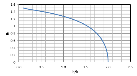
(10) It is noticed that the ratio RR is independent of a and b but h/b only. Table 2 and Figure 4 present the RR data in the full range of b h/ . They indicate that RR=_1 occurs at _h/b=1.54. Figure 5 shows the two cross sections for h/b=1.54. Since RR=_1 does not hold true at other _h/b ratio values, Bourgoyne, et al. [15] slot cross-section model is not valid for channels with bow-shaped cross sections. The error of Bourgoyne et al.’s model is expressed as
1 1 1 1 p p slot bow EB p p R bow R bow pslot
$$ = \frac {\Delta p _ {s l o t} - \Delta p _ {b o w}}{\Delta p _ {b o w}} = \frac {1}{\underline {{\Delta p _ {b o w}}}} - 1 = \frac {1}{R _ {R}} - 1 $$ (11) ∆ where EB is the relative error of Bourgoyne et al.’s model, D_p_slot is the pressure gradient given by Bourgoyne et al.’s model [15], and D_p_slot is the pressure gradient given by Equation (4). For channels with flat cross sections where h/ b<1.0, the RR value varies from 1.27 to 1.50. These RR values are translated by Equation (11) to -21% and -33% relative error, respectively.
| h/b | RR | h/b | RR |
|---|---|---|---|
| 0.1 | 1.5 | 1.55 | 0.99 |
| 0.2 | 1.48 | 1.56 | 0.98 |
| 0.3 | 1.45 | 1.59 | 0.96 |
| 0.4 | 1.43 | 1.62 | 0.93 |
| 0.5 | 1.41 | 1.67 | 0.89 |
| 0.6 | 1.39 | 1.72 | 0.83 |
| 0.7 | 1.36 | 1.77 | 0.77 |
| 0.8 | 1.34 | 1.82 | 0.69 |
| 0.9 | 1.31 | 1.87 | 0.6 |
| 1 | 1.27 | 1.92 | 0.49 |
| 1.1 | 1.24 | 1.93 | 0.46 |
| 1.2 | 1.2 | 1.94 | 0.43 |
| 1.3 | 1.15 | 1.95 | 0.39 |
| 1.4 | 1.09 | 1.96 | 0.35 |
| 1.45 | 1.06 | 1.97 | 0.31 |
| 1.5 | 1.03 | 1.98 | 0.25 |
| 1.51 | 1.02 | 1.99 | 0.22 |
| 1.52 | 1.01 | 1.99 | 0.18 |
| 1.53 | 1.01 | 2 | 0.13 |
| 1.54 | 1 | 2 | 0 |
Table 3: Model-calculated data of _h/b_ versus _R__R__._
| w | |
| a | |
| b |
Table 6: Model-calculated data of _h/b_ versus _R__R__._
| w |
|---|
Table 7: Model-calculated data of _h/b_ versus _R__R__._
Bow-shape
Cross Section
| h | |
|---|---|
Table 8: Model-calculated data of _h/b_ versus _R__R__._
Case Analysis
This section shows an application of the newly developed hydraulics model in a cement squeezing operation. The objective is to seal a channel behind casing without break down the formation.
A primary cement job has been performed on a 7” production casing. After 48 hours wait on cement time, a cement bond log was run. Result of log interpretation indicated that a long channel exists in the annulus. The volume of the channel is about 5% of the annulus space over the logged interval. A cement squeezing operation is designed as shown in Figure 6. The cement slurry is designed to have a weight of 15.8 ppg with flow consistency K=30 cp equivalent and flow behavior index n=0.95. The placement efficiency of cement in the channel depends on cement properties and cement slurry flow velocity during cement squeezing. It is essential to know the maximum permissible pumping rate that will not induce friction pressure to break down the formation. It is also essential to know the peak surface pumping pressure corresponding to the formation fracturing pressure at bottom hole so that the pumping rate is monitored and controlled to avoid formation break down.
10 ppg polymer drilling fluid
10-3/4 in. OD, 40.5 lb/ft casing
9,350 ft
10 ppg NaCl brine
25 bbl Spacer
2-7/8 in. EUE tubing
9,325 ft
9-5/8 in. borehole Packer
Channel behind casing
5 bbl spacer
20 bbl 15.8 ppg cement slurry
9,800 ft Fracture gradient 0.8 psi/ft Perforations:4 shots/ft,
360 deg. phasing
9,850 ft
7-in. OD, 26-lb/ft casing
10,000 ft Figure 6: Schematic of a cement squeezing design.
The annulus area is
$$ A _ {a} = \frac {\pi}{4} \left[ \left(9. 6 2 5\right) ^ {2} - \left(7\right) ^ {2} \right] = 3 2. 2 6 \mathrm {i n} ^ {2} $$ The cross sectional area of the channel is estimated to be (0.05)(34.26) = 1.71 in2 Assuming bow-shape cross section of the channel, the height of the cross section can be estimated using Equation (2):
( ) ( ) ( ) ( )
9.625 / 2
9.625 / 2
$$ 1 = \frac {9 . 6 2 5 / 2}{9 . 6 2 5 / 2} \left[ \frac {\pi}{2} \left(9. 6 2 5 / 2\right) ^ {2} + \left(h - 9. 6 2 5 / 2\right) \sqrt {2 h \left(9. 6 2 5 / 2\right) - h ^ {2}} + \left(9. 6 2 5 / 2\right) ^ {2} \arcsin \left(\frac {h - 9. 6 2 5 / 2}{9. 6 2 5 / 2}\right) \right] $$
which gives h = 0.57 in.
The formation fracturing pressure can be predicted using formation fracture pressure gradient 0.8 psi/ft and depth at the bottom of channel:
$$ p _ {F} = (0. 8) (9, 8 5 0) = 6, 3 0 4 \mathrm {p s i} $$
The flowing cement pressure at the bottom of the channel is:
(0.052)(10)(9,350) (0.052)(15.8)(9,850 9,350) p p C f p f $$ = (0. 0 5 2) (1 0) (9, 3 5 0) + (0. 0 5 2) (1 5. 8) (9, 8 5 0 - 9, 3 5 0) + $$
5,273 = + Equating PF and PC yields maximum permissible friction pressure of cement slurry pf = 1,031 psi, which gives pressure gradient of dpf /dz = (1,031)/(9,850-9,350) = 2.06 psi/ft. Table 3 presents a summary of calculations given by Equation
(4). It shows that the maximum permissible pumping rate is 4.33 bpm. For safe operations the cement pressure should be controlled to be lower than the formation breakdown pressure by at least 500 psi. Therefore a pumping rate of 2 bpm is recommended for this operation. This pumping rate is expected to create a frictional pressure of 495 psi in the channel, as shown in Table 3.
| Q (bpm) | vav (ft/s) | ma (cp) | dpf/dz (psi/ ft) | pf (psi) |
|---|---|---|---|---|
| 0.5 | 3.9 | 21.6 | 0.27 | 133 |
| 1 | 7.9 | 20.9 | 0.51 | 256 |
| 1.5 | 11.8 | 20.5 | 0.75 | 376 |
| 2 | 15.7 | 20.2 | 0.99 | 495 |
| 2.5 | 19.7 | 20 | 1.22 | 612 |
| 3 | 23.6 | 19.8 | 1.45 | 727 |
| 3.5 | 27.5 | 19.6 | 1.68 | 842 |
| 4 | 31.5 | 19.5 | 1.91 | 956 |
| 4.33 | 34.1 | 19.4 | 2.06 | 1,031 |
| 4.5 | 35.4 | 19.4 | 2.14 | 1,069 |
| 5 | 39.3 | 19.3 | 2.36 | 1,181 |
Table 9: Result of Calculations Given by Equation (4).
When the frictional pressure of 495 psi is added to the hydrostatic pressure in the channel, the pressure at the bottom of the channel becomes 5,273+495=5,768 psi. This corresponds to a surface squeezing pressure of 5,768- 0.052(10)(9,850) =646 psi. The surface “breakdown” pressure is calculated to be $$ p _ {b d} = (0. 8) (9, 8 5 0) - (0. 0 5 2) (1 0) (9, 8 5 0) = 2, 7 5 8 \mathrm {p s i} $$ This pressure is the optimum breakdown pressure. Breakdown can occur at lower pressures depending on the number of opened perforations, increased efficiency with higher viscosity, etc.
Conclusions
A new analytical model was developed in this project to describe fluid flow in channels behind well casing. The model assumes general bow-shaped cross sections of flow channels. The following conclusions are drawn.
- The new model is equivalent to the Bourgoyne, et al. [15] slot model only for channel parameter h/b=1.54, indicating a limitation of Bourgoyne, et al. model to channels with special geometries. For channel parameter h/b<1.54, use of Bourgoyne, et al. model should under- estimate pressure gradient in channels; while for channel parameter h/b>1.54, use of Bourgoyne, et al. model should over-estimate pressure gradient in channels [15].
- For channels with narrow cross sections (h/b<
Nomenclature
A = area of bow-shaped cross-sections, in2 a = half-length of the long axis of the ellipse, in b = half-length of the short axis of the ellipse, in F1 = force applied by the fluid pressure at Point 1, pound F2 = force applied by the fluid pressure at Point 2, pound F3 = frictional force exerted by the adjacent layer of fluid below the fluid element of interest, pound F4 = frictional force exerted by the adjacent layer of fluid above the fluid element of interest, pound h = height of bow-shaped cross-section, in Κ = fluid consistency index, cp equivalent n = flow behavior index p = pressure, pound per square inch (psi) pf = frictional pressure, psi pF = formation fracturing pressure, psi pC = flowing cement pressure at the bottom of the channel, psi pbd = surface “breakdown” pressure, psi Q = volumetric flow rate, ft3/s R = radius of the circle, in RR = resistance ratio v = flow velocity, ft/s vav = average velocity, ft/s v0 = velocity at boundary, ft/s w = width of cross-section, in weq = equivalent width of cross section, in x = horizontal coordinate of ellipse y = vertical coordinate of ellipse Dy = thickness of fluid element, in z = horizontal coordinate in the flow direction Dz = length of the fluid element, in Greeks γ = shear rate, s-1 m = Newtonian viscosity, cp ma = apparent viscosity, cp mp = plastic viscosity, cp τ = shear stress, lb/ft2 t0 = shear stress at boundary, lb/ft2 ty = yield point, lb/100 ft2
Acknowledgment
This research was supported by the U.S. - Israel Center of Excellence in Energy, Engineering and Water Technology through the project “Safe, sustainable, and resilient development of offshore reservoirs and natural gas upgrading through innovative science and technology: Gulf of Mexico – Mediterranean.”
References
-
Uswak G, Howes E (1992) Direct Detection of Water Flow behind Pipe Using A Transient Oxygen Activation Technique. Journal of Canadian Petroleum Technology 31(4): 9.
-
Dossary A, Al-Majed AA, Hossain E, Rahman MK, Jennings SS, et al. (2011) Cementing at High Pressure Zones in KSA “Discovering the Mystery Behind the Pipe.” SPE Middle East Oil and Gas Show and Conference, Society of Petroleum Engineers, Manama, Bahrain, pp: 13.
-
Duguid A, Guo B, Nygaard R (2017) Well integrity assessment of monitoring wells at an active CO2-EOR flood. 13th International Conference on Greenhouse Gas Control Technologies (GHGT-13), Lausanne, Switzerland, pp: 5119-5138.
-
Marca C (1990) 13 Remedial Cementing. Developments in Petroleum Science 28: 13-1-13-28.
-
Bakulin A, Korneev V (2007) Acoustic Signatures of Cross-flow Behind Casing: Downhole Monitoring Experiment At Teapot Dome. Society of Exploration Geophysicists, San Antonio, Texas.
-
Perrier S (2011) Detection of Cross-flows Behind Casing before Perforations, and Cement Isolation Diagnosis Based on Temperature Analysis (TUNU field, Indonesia). International Petroleum Technology Conference. Bangkok, Thailand, pp: 19.
-
Croon M, Huber P, Wright J (2019) Enhanced Well Remedial Decisions from Exact Location of Fluid Movement Behind Casing Identification. Abu Dhabi International Petroleum Exhibition & Conference, Society of Petroleum Engineers, Abu Dhabi, UAE, pp: 16.
-
Grant WH, White RL, Smith RC, Miller AG (1990) Successful Squeezing of Shallow and Low-Pressure Formations. IADC/SPE Drilling Conference, Society of Petroleum Engineers, Houston, Texas, pp: 8.
-
Saponja J (1999) Surface Casing Vent Flow And Gas Migration Remedial Elimination-New Technique Proves Economic And Highly Successful. Petroleum Society of Canada, Calgary, Alberta, pp: 17.
-
Slater HJ (2010) The Recommended Practice for Surface Casing Vent Flow and Gas Migration Intervention. SPE Annual Technical Conference and Exhibition, Society of Petroleum Engineers, Florence, Italy.
-
Jabarov KA (2019) Mathematical modeling the processes of behind-casing fluid movement in the wells during waiting on cement (Russian). Oil Industry Journal 2019(5): 5.
-
Goodwin KJ, Crook RJ (1992) Cement Sheath Stress Failure. SPE Drill Eng 7(4): 291-296.
-
Tamayol A, Bahrami M (2010) Laminar Flow in Microchannels With Noncircular Cross Section. Journal of Fluids Engineering 132(11): 111201.
-
Wu B (2014) The influence of the cross section shape on channel flow: modeling, simulation and experiment. Modeling and Simulation. Université de Grenoble, France, pp: 252.
-
Bourgoyne AT, Millheim KK, Chenevert ME, Young FS (1986) Applied Drilling Engineering. Volume 2, SPE textbook series, Society of Petroleum Engineers, Richardson, Texas, USA, pp: 137-144.
-
Guo B, Liu G (2011) Applied Drilling Circulation Systems_._ Gulf Professional Publishing_,_ Elsevier, pp: 272.
- Nigeria’s Vulnerability in the Face of Global Energy Policy
- A Simulation Study of Investigation of Optimum Oil Production Performance by Applying Various Gas Injection Methods in Oil Reservoir
- Characterization of Permo-Triassic Reservoirs through Thermal Maturity Assessment of Westphalian Source Rocks in the Cheshire Basin
- Influence of Microwax on the Rheological and Thermal Behaviour of a Wax Crude Oil
- Real-Time Monitoring and Performance Optimization of Steam Injection in Heavy Oil Reservoirs Using Fiber Optic Sensing and Integrated Predictive Simulation Models
- Rapid On-Site Determination of the Total Petroleum Hydrocarbon Content of Soils by Handheld Fourier Transform Near-Infrared Spectroscopy: Development of a Global, Site- and Scanner- Independent Calibration Model