Determination of Pressure Fluctuations in the Wellbore During Drilling Operations

Solution of the Problem

The loading and discharge stages of the volcanic viscous- plastic mountain rocks can be written according to the following differential equations (4):

For the loading process

$$m_l \frac{d^2 \theta_l}{dt^2} + \eta_l \frac{d\theta_l}{dt} + k_l \theta_l \leq P_l - P_s - \sigma_{fr} \tag{1}$$

For the unloading process

$$m_{ul} \frac{d^2 \theta_{ul}}{dt^2} + \eta_l \frac{d\theta_{ul}}{dt} + k_{ul} \theta_{ul} \leq P_{ul} - P_s - \sigma_{rt} \tag{2}$$

Here and there $\theta_l$ and $\theta_{ul}$ – respectively, relative dimensional deformations for loading and unloading processes; $P_{l}, P_{ul}$ – pressures arising from appropriate processes; $k_l, k_{ul}$ – are volume compression modules in these processes; $P_s$ – side pressure of mountain rocks; $\sigma_{fr}$ – resistance to hydraulic fracturing of mountain rocks; $\sigma_{rt}$ – resistance of mountain rocks to tension; $m_l = \frac{\pi D}{g} P_l, m_{ul} = \frac{\pi D}{g} P_s$ – are the masses brought into the unit length of the borehole; $D$ – Diameter of well; $g$ – acceleration of gravity; $\eta_k$ – respectively, the coefficients that characterize the viscosity and elasticity of mountain rocks. In general, the relative volume deformation of the rocks is defined as the power function of the pressure in the borehole:

$$\theta_l = a P^{b_1} \tag{3}$$

If the loading process is with residual deformation, then

$$\theta_{ul} = \theta_0 + a_1 P_{ul}^{b_1} \tag{4}$$

Thus, the equilibrium equation of viscous-elastic mountain rocks (including some sands, marls, shale etc.) in well conditions can be expressed by the following equation:

$$m\theta''(t) + \eta\theta'(t) + k\theta(t) + P_s - P_{fr} - \Delta P = 0 \tag{5}$$

Equation (5) represents a homogenous viscous-elastic environment model of mountain rocks and their direct contact with neutral drilling mud. The physical and mechanical interaction of mountain rocks with drilling mud is different and has not been studied until now.

It is well known that the pressure drop in the borehole can be designated as

$$\Delta P = \gamma H - P_{rl} + P_{add} \tag{6}$$

Here is:

$$\gamma - \text{the specific gravity of the drilling mud}; H \text{ depth of well;}$$

$$P_{rl} - \text{reservoir layer pressure}; P_{add} - \text{an additional pressure that occurs in annular space.}$$

Usually this pressure is assumed to be constant [4]. In fact, the pressure of the drilling mud changes in a annular space while performing various technological processes in the drilling process. Therefore, the following approximate dependencies can be assumed to change this pressure:

$$\Delta P = \gamma H - P_{rl} + P_{add} \tag{7}$$

$$P_{add} = c \cos \omega t,$$

Where $c$ and $\omega$ – the amplitude and frequency of additional pressure changes, respectively. In general, the pressure changes in an annular space can be represented as the Fourier series:

$$P_{add}(l, t) = \sum_{n=1}^{\infty} A_n \exp(i\omega t) \tag{8}$$

$$A_n = \frac{\omega}{2\pi} \int_{\frac{\pi}{\omega}}^{0} f(t) \exp(i\omega t) dt, \quad (n = 0; \pm 1; \pm 2...) \tag{9}$$

For simplifications, we accept that these variables are subject to the expression (7). If we take (6) and (7) into account (5)

$$(A + B \cos \omega t) \theta''(t) + \eta\theta'(t) + k\theta(t) = F(t) \tag{10}$$

In the equation (10)

$$A = \frac{\pi D}{g} \left( \gamma H - P_{rl} \right),$$

$$B = \frac{\pi D c}{g}, \tag{11}$$

$$F(t) = P_{fr} + \gamma H - P_s - P_{rl} - c \cos \omega t.$$

Thus, it is clear that the dynamic stability of the mountain rocks around the well is represented by a heterogeneous equations with variable and periodic coefficients.

The homogeneous periodic solution of equations (10) with a periodicity of 2T is being sought the following equation:

$$\theta(t) = a_1 \sin \frac{\omega t}{2} + b_1 \cos \frac{\omega t}{2} + \dots \tag{12}$$

Given the equation (12) in the homogeneous equation and zeroing the coefficients $\sin k\omega t$ vs $\cos k\omega t$ of the same set, we construct the system of algebraic equations below:

2 2 1 0, 1 1 4 2 4 2

$$ 1 \left(k - A \frac {\omega^ {2}}{4} + \frac {1}{2} B \frac {\omega^ {2}}{4}\right) - b _ {1} \eta \frac {\omega}{2} = 0 $$ ω ω ω η a k A B b (13)

2 2 1 0. 1 1 4 2 4 2

$$ 1 \left(k - A \frac {\omega^ {2}}{4} - \frac {1}{2} B \frac {\omega^ {2}}{4}\right) - a _ {1} \eta \frac {\omega}{2} = 0 $$ ω ω ω η b k A B a The existence of periodic solutions of the homogeneous equation different from zero is conditioned by the fact that the determinant of the conditional system (13) is zero. Using this condition, we obtain the following critical frequencies equation:

2 2 2 1 4 2 4 4 0 2 2 2 1 4 4 2 4

ω ω ω η k A B

$$ \left. \begin{array}{c c c c} \kappa - A \frac {\omega^ {2}}{4} + \frac {1}{2} B \frac {\omega^ {2}}{4} & - \eta \frac {\omega^ {2}}{4} \\ 2 & 2, & 2 \end{array} \right| = 0 $$ (14) ω ω ω η k A B − − From the determinant

4 2 2 2 4 2 2 4 4 1,2 2 2 0,25

kA k B kA

$$ \omega_ {1, 2} = \sqrt {\frac {4 k A - 2 \eta \pm 2 \sqrt {\eta^ {4} + 4 k ^ {2} B ^ {2} - 4 k A \eta^ {2}}}{A ^ {2} - 0 , 2 5 B ^ {2}}} $$ (15) A B For all of the values ​within the range defined by the formula (15), the amplitudes obtained from the homogeneous equation solutions are infinitely increasing. The formulas (15) allow to define the amplitude and frequency of the additional pressure changes in the annular space, which causes the volatile state of the wells borehole, that is the contractions, leaks and spikes in the borehole are inevitable in these pressure changes. For absolute elastic rocks, that is, for the case η = 0 [7].

( ) 2 1,2 2 2 0,25

k A B

$$ \omega_ {1, 2} = 2 \sqrt {\frac {k (A \pm B)}{A ^ {2} - 0 , 2 5 B ^ {2}}} $$

(16) It means that for absolute elastic rocks, there is also an amplitude and frequency of additional pressure in the annular space, which causes instability.

The following linear algebraic equations system as a result of the homogeneous solution for periodicity of T:

2 0 0,5 0, 0 2 2 2 0 0, 0 2 2 2 0 0. 0 2 2

k b a B b ω $$ k \cdot b _ {0} - 0 \cdot a _ {2} - 0, 5 \cdot B \cdot \omega^ {2} \cdot b _ {2} = 0 $$ ( ) b k A a b ω ηω ⋅ + − ⋅ − = (17) ( ) b a k A b ηω ω ⋅ + + − ⋅ = And as a result the solution of its determinant

2 0 0,5 2 0 0 2 0

k B ω − (18) k A

ω ηω $$ x - A \omega^ {2} \quad - \eta \omega \quad = 0 $$

k A ηω ω − For determining of the boundaries first instability area on changes the frequency the following expression is received:

The analysis conducted was based on models that assumed linear variation of parameters. If the models include ξ −nonlinear viscosity coefficients and γ −nonlinear elasticity coefficients, instead of the first homogeneous equation may be used the equation with the nonlinear coefficients:

$$ \left(A + B \cos \omega t\right) \theta^ {\prime \prime} + \eta \theta^ {\prime} + \xi \theta^ {1} \theta^ {2} + k \theta + \gamma \theta^ {3} = 0 \tag {20} $$ The solution of equation (20) can be searched as 2T or T periodicity series like (12). For this purpose, at first the non- linear assemblies are divided into Fourier series.

For periodic solutions with 2T periodicity $$ \xi \theta^ {1} \theta^ {2} + \gamma \theta^ {3} = \Phi \left(a _ {1} b _ {1}\right) \sin \frac {\omega t}{2} + \psi \left(a _ {1} b _ {1}\right) \cos \frac {\omega t}{2} + \dots , \tag {21} $$

4 1 1 2 3 sin , 1 1 2 2 0 4 1 1 2 3 cos . 1 1 2 2 0

πω ω ω ξθ θ γθ π πω ω ω ψ ξθ θ ηθ π $$ \left. \begin{array}{l} \Phi \left(a _ {1} b _ {1}\right) = \frac {\omega}{2 \pi} \int_ {0} ^ {4 \pi \omega - 1} \left(\xi \theta^ {1} \theta^ {2} + \gamma \theta^ {3}\right) \sin \frac {\omega t}{2} d t, \\ \psi \left(a _ {1} b _ {1}\right) = \frac {\omega}{2 \pi} \int_ {0} ^ {4 \pi \omega - 1} \left(\xi \theta^ {1} \theta^ {2} + \eta \theta^ {3}\right) \cos \frac {\omega t}{2} d t. \end{array} \right| $$ ( ) ( ) t a b dt (22) ( ) ( ) t a b dt For the reports based on (21) and (22) equations ( ) ( ) 2 2 1 2 3 3 sin 3 cos ..., 1 1 1 1 4 2 4 2 2 2 2. `1 1 a t a t a b b a $$ \xi \theta^ {1} \theta^ {2} + \gamma \theta^ {3} = \frac {a ^ {2}}{4} \left(3 \gamma a _ {1} + \xi \omega b _ {1}\right) \sin \frac {\omega t}{2} + \frac {a ^ {2}}{4} \left(3 \gamma b _ {1} + \xi \omega a _ {1}\right) \cos \frac {\omega t}{2} +.. $$ (23) a a b = + Substituting (21) and (22) in to (20) and if we accept the coefficients on sin k t ω və cos_k t_ ω equal to zero, then

2 2 2 1 3 0, 1 1 1 1 4 2 4 4 4

    − + − + − =         − − + + − =    

a a k A B b a b

( ) ω ω ω η γ ξω (24)

The condition of the existence of solutions of the system (24) that is different from zero is that its determinant is zero, i.e

2 2 2 2 1 3 4 4 2 4 2 4 0 2 2 2 2 1 3 2 4 4 4 2 4

a a k A B ω ω ω γ η ξω $$ \left| \begin{array}{c c c c} \kappa - A \frac {\omega^ {2}}{4} + \frac {a ^ {2}}{4} 3 \gamma + \frac {1}{2} B \frac {\omega^ {2}}{4} & - \eta \frac {\omega}{2} - \frac {a ^ {2}}{4} \xi \omega & & \\ 2 & 2 & 2 & 2 \end{array} \right| = 0 $$ a a k A B ω ω ω η ξω γ $$ \frac {1}{2} + \frac {a ^ {2}}{4} \xi \omega \quad k - A \frac {\omega^ {2}}{4} + \frac {a ^ {2}}{4} 3 \gamma - \frac {1}{2} $$ (25) From the solution of the determinant, we determine that

where

2 2 6 1,5 , 1 2 2 2 9 ,

g k A γ ηξω γω $$ = 6 \gamma k + \eta \xi \omega^ {2} - 1 $$

(27) P γ γ ω = +

1 1 1 1 2 2 2 2 2 4 2 4 2 4 16 64

l k k A A B

ω η ω ω ω $$ l = k ^ {2} - \frac {1}{2} k \omega^ {2} A + \frac {1}{4} \eta^ {2} \omega^ {2} + \frac {1}{1 6} A ^ {2} \omega^ {4} - \frac {1}{6} $$ Equations (25) and (26) determine the amplitude- frequency dependence of the main variables of equation (20).

Unstable solutions of the equation of (20) are characterized by a lower curve of the resonance curve. Equation of (20) shows that if nonlinear constants are eliminated, then the unsteady solutions are defined by the boundaries of linear theory, i.e., equations (15) and (16).

Let’s investigate the coordinated mode of changes near the main resonance. The solving equation of (20) looking for as under mentioned $$ \theta (t) = a (t) \sin \frac {\omega t}{2} + b (t) \cos \frac {\omega t}{2} + \dots , \tag {28} $$ Here are ( ), ( ) a t b t −” weakly changing functions”, that is, these are less time-varying coefficients. Considering series of (28) and its first and second derivatives in equation (20), and after intermediate transformations received decisions we can construct the following equation system:

( )( ) ( ) ( )

2 0,5 0,25 0,5 , 0,

$$ 4 - 0, 5 B) \left(a ^ {\prime \prime} - \omega b ^ {\prime} - 0, 2 5 \omega^ {2} a\right) + \eta \left(a ^ {\prime} - 0, 5 \omega b\right) + k a + \Phi (a, b) = 0 $$ A B a b a a b ka a b ω ω η ω (29) ( )( ) ( ) ( )

2 0,5 0,25 0,5 , 0.

′′ ′ ′ + + − + + + + Φ =

A B b a b b a kb a b ω ω η ω The system of equations (29) can be simplified according to the requirements of the method of “ less variable functions”. For this reason, if we do not take into account second-order small slogans, then ( )( ) ( )

2 0,5 0,25 , 0,5 ,

$$ 4 - 0, 5 B) \left(0, 2 5 \omega^ {2} a + \omega b ^ {\prime}\right) = \Phi (a, b) + k a - 0 $$ A B a b a b ka b ω ω ηω (30) ( )( ) ( )

2 0,5 0,25 , 0,5 .

$$ 4 + 0, 5 B) \left(0, 2 5 \omega^ {2} b - \omega a ^ {\prime}\right) = \psi (a, b) + k b + 0 $$ A B b a a b kb a ω ω ψ ηω Equation of (30) shows that the ratio used for the steady state can be obtained from values $$ a ^ {\prime} (t) = b ^ {\prime} (t) = 0 \mathrm {[ 3 1 ]} $$ By excluding non-linear assemblies in system of (30) for the pre - steady state under mentioned values ( ) exp( ) a t ht α = = (32) ( ) exp( ) b t ht β can be used, where , ,h α β −are constant coefficients.

Given the expression (32) in (30), we have the following system of equations

2 0,5 0,25 0,5 0, $$ \begin{array}{l} \left[ \left(A - 0, 5 B\right) 0, 2 5 \omega^ {2} - k \right] \alpha + \left(\omega h + 0, 5 \eta \omega\right) \beta = 0 \\ \left[ \left(A + 0, 5 B\right) 0, 2 5 \omega^ {2} - k \right] \beta - \left(\omega h + 0, 5 \eta \omega\right) \alpha = 0 \\ \end{array} $$ ( ) ( ) A B k h ω α ω ηω β (33)

2 0,5 0,25 0,5 0.

( ) ( ) A B k h

ω β ω ηω α We can set an index of increase (decrease) given the existence of solutions other than zero like (32):

$$ h = \pm \sqrt {0 , 0 1 5 6 2 5 B ^ {2} \omega^ {2} - \left(0 , 2 5 A - \frac {k}{\omega}\right) ^ {2}} - 0, 5 \eta $$ (34) h −positive values correspond to an increase of the steady changes amplitude and the negative values to an its decrease.

As a result, studies to clarify the effect of changes in reverse pressures on the deformation of rocks [6] have shown that there are three characteristic parts of the deformation curves of the samples:

Area of unstable deformations, area of steady deformation and area of intensity of viscous-plastic deformations.

It is likely that the identified deformations will be characteristic of a number of rocks in general. Thus, it is possible to determine the coefficients k and η, using the results of the above analysis, to determine the deformation regimes that can occur with rocks and to develop proposals for their elimination.

In order to continue the study of mountain rock instability (10) let us determine the relative changes in volume relative deformation based on the solution of equation. Write this equation explicitly [3, 6]:

$$\left( A + B \cos \omega t \right) \theta''(t) + \eta \theta'(t) + k \theta(t) = d + c \cos \omega t$$

$$d = \sigma_{qr} + \gamma H - P_B - P_{lay}$$

and seek its solution as follows:

"2T" periodic solutions

$$\theta(t) = \sum_{n=1}^{\infty} \left( x_n \cos \frac{\omega t}{n} + y_n \sin \frac{\omega t}{n} \right),$$

"T" periodic solutions

$$\theta(t) = \sum_{n=1}^{\infty} \left( x_n \cos n \omega t + y_n \sin n \omega t \right),$$

$x_n, y_n$ are the coefficients determined by the joint solution of equations (35), (37) and (38).

Let us investigate the characteristic case with periodic variations of "T". (38) We find that

$$\theta'(t) = \sum_{n=1}^{\infty} n \omega \left( y_n \cos n \omega t - x_n \sin n \omega t \right),$$

$$\theta''(t) = \sum_{n=1}^{\infty} n \omega^2 \left( x_n \cos n \omega t + y_n \sin n \omega t \right),$$

Considering (38) - (40) in (35), we create an infinite linear algebraic equation system for $x_n, y_n$ to sum the coefficients $\cos k \omega t$ vs $\sin k \omega t$ to zero:

$$x_n, y_n;$$

$$\left( k - \omega^2 A \right) x_1 - \eta \omega y_1 - \omega^2 B \left( 4 \cdot \frac{1}{2} x_2 \right) = c,$$

$$\left( k - \omega^2 A(4) \right) x_2 - \eta \omega 2 y_2 - \omega^2 B \left( 1 \cdot \frac{1}{2} x_1 + 9 \cdot \frac{1}{2} x_3 \right) = 0,$$

$$\left( k - \omega^2 A(9) \right) x_3 - \eta \omega 3 y_3 - \omega^2 B \left( 4 \cdot \frac{1}{2} x_2 + 16 \cdot \frac{1}{2} x_4 \right) = 0,$$

$$\left( k - \omega^2 A(n) \right) x_n - \eta \omega(n) y_n - \omega^2 B \left( (n-1)^2 \cdot \frac{1}{2} x_{n-1} + (n+1)^2 \cdot \frac{1}{2} x_{n+1} \right) = 0,$$

$$\left( k - \omega^2 A \right) y_1 - \eta \omega x_1 - \omega^2 B \left( 4 \cdot \frac{1}{2} y_2 \right) = 0,$$

$$\left( k - \omega^2 A(4) \right) y_2 - \eta \omega x_2 - \omega^2 B \left( 1 \cdot \frac{1}{2} y_1 + 9 \cdot \frac{1}{2} y_3 \right) = 0,$$

$$\left( k - \omega^2 A(9) \right) y_3 - \eta \omega x_3 - \omega^2 B \left( 4 \cdot \frac{1}{2} y_2 + 16 \cdot \frac{1}{2} y_4 \right) = 0,$$

$$\left( k - \omega^2 A(n)^2 \right) y_n - \eta \omega(n) x_n - \omega^2 B \left( (n-1)^2 \cdot \frac{1}{2} y_{n-1} + (n+1)^2 \cdot \frac{1}{2} y_{n+1} \right) = 0.$$

There is a simple solution of the system of equations (41) for absolute elastics (status $\eta = 0$) mountain rocks:

$$x_1 = -\frac{2d}{B \omega^2},$$

$$x_2 = \frac{\left( k - A \omega^2 \right) x_1 - c}{2B \omega^2},$$

$$x_3 = \frac{2 \left( k - 4 A \omega^2 \right) x_2 - \frac{1}{2} x_1},$$

$$x_4 = \frac{2 \left( k - 9 A \omega^2 \right) x_3 - \frac{4}{16} x_2},$$

$$x_n = \frac{2 \left[ k - (n-1)^2 A \omega^2 \right] x_{n-1} - \left( \frac{n-2}{n} \right) x_{n-2}}{n = 5, 6 \dots}$$

In the end result (41) defines a reactive approach to solving the system.

It is also necessary that the deformation changes $n \rightarrow \infty$ - da $x_n \rightarrow \infty$ are stable. From the last (42) formula to paying for this condition

$$\frac{2 \left[ k - (n-1)^2 A \omega^2 \right]}{n^2 B \omega^2} < 1$$

Anticipation of inequality is necessary and sufficient.

The latter is conditional, and this result can be used to solve technological issues. Let's test the appropriateness of the mathematical dependence obtained on the following data. Assuming that mountain rocks are also composed of clay shale, for that $k = 3 \times 10^3$ MPa; $\eta = 3 \times 10^3$ MPa; $c$ density of drilling mud - $\rho = 1880$ kg/m$^3$; well diameter - is 190 mm; perpetration - $\gamma H - P_{rz} = 70$ MPa; $C = 2000$ MPa; $k = 0.1 \times 10^6$ MPa; $d = 800$ MPa; $\omega = 6 \times 10^3$ [8, 9].

For these parameter values, is determined that $A = 4.86$ and $B = 12.16$.

From the system of equations (42)

$$x_1 = -0.365;$$

$$x_2 = -4.330;$$

$$x_3 = -20.403;$$

$$x_4 = -48.000;$$

$$x_5 = -55.819;$$

$$x_6 \dots x_{15} = 4.064;$$

$$x_{25} = 0.883;$$

$$x_{35} = -0.319.$$

The relative volume rock deformation for its stationary changes (for $\eta = 0$ condition) can be written according (38)

Click to enlarge

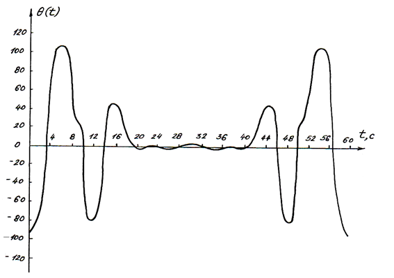
The obtained results allow estimation of the velocity and amplitude characteristics of the well pressure change, which prevents the process of rock erosion (i.e, preventing the well wall from collapsing and collapsing on the wall itself).

References

-
Basarigin YM, Budnikov VF, Bulatov AI, Geraskin VG (2000) Construction of inclined and horizontal wells. Nedra, Moscow, pp: 262.
Gilyazev RM (2002) Oil well drilling with sidetracks. Nedra, Moscow, pp: 255.
Lechnitski SG (1977) The theory of elasticity of an anisotropic body. Science, pp: 416.
Seid Rza MK, Farajev TG, Hasanov RA (1992) Prevention of complications in the kinetics of drilling processes. Nedra, Moscow, pp: 325.
Stokely KO (1991) Improving the efficiency of horizontal drilling in fractured carbonates. Oil, gas and petrochemicals abroad 10: 61-68.
Cherepanov GP (1987) Mechanics of rock destruction during drilling. Nedra, Moscow, pp: 308.
Shirali I, Hasanov R, (2017) Drilling of the wells: Innovative technics and technology. Lambert Academic publisher, Germany, pp: 378.
Hasanov RA, Shirali IY, Kazimov MI (2020) Determination of the amplitude–frequency Characteristics of the well pressure preventing the destruction of wellbore rocks. Global Journal of Science Frontier Research 20(1): 36- 42.
Yan C, Deng J, Yu B, Liu H, Deng F, et al. (2018) Wellbore stability analysis and its application in the Fergana basin, central Asia. US department of energy, office of Science.
- Nigeria’s Vulnerability in the Face of Global Energy Policy
- A Simulation Study of Investigation of Optimum Oil Production Performance by Applying Various Gas Injection Methods in Oil Reservoir
- Characterization of Permo-Triassic Reservoirs through Thermal Maturity Assessment of Westphalian Source Rocks in the Cheshire Basin
- Influence of Microwax on the Rheological and Thermal Behaviour of a Wax Crude Oil
- Real-Time Monitoring and Performance Optimization of Steam Injection in Heavy Oil Reservoirs Using Fiber Optic Sensing and Integrated Predictive Simulation Models
- Rapid On-Site Determination of the Total Petroleum Hydrocarbon Content of Soils by Handheld Fourier Transform Near-Infrared Spectroscopy: Development of a Global, Site- and Scanner- Independent Calibration Model