The Bakken and Three Forks Formations Daily Crude Oil Production per Well Prediction Based on Support Vector Regression
In the oil and gas industry, there is a major challenge to accurately predict the crude oil production due to the complexity and sophistication of the subsurface conditions. Production forecasting is highly limited by the non-linearity between hydrocarbon production and any relevant petrophysical parameter. Trying to use just the conventional mathematical approaches might give inaccurate result because of the numerous assumptions employed by this approach. Therefore, there is a huge need to develop a reliable prediction model of hydrocarbon production. This will surely assist Petroleum Engineers to have a better understanding of the entire reservoir behavior to solve, evaluate, and optimize its overall performance. Utilizing data driven models which is the machine learning techniques can help to predict crude oil production with much more acceptable accuracy. In this paper, Python-Support Vector Regression and Orange-Linear Regression have been implemented to build the models that predict the daily oil production of a well in Bakken-Three Forks Formations. The statistical data for the Bakken-Three Forks formation oil production was from North Dakota Industrial Commission (NDIC) website. An open-source visual programmingbased data mining software Orange was used to train a multi-linear regression model of 817 datasets with addition of 200 lines of code algorithm written in Python which is a high-level programming language. Combination of these two software models gave a more robust and accurate predictions compared to the conventional method of using just a software model by others. The models developed can practically estimate the Daily oil production of a well in Bakken-Three Forks Formations. The R2 obtained is 0.98 from the low performance value of 0.35, the MAE became 10.593 and RMSE is 16.593 for SVR and linear regression with a cross validation of 10 folds for the 70% train dataset and 30 % test dataset shows MSE value of 2.826, RMSE of 1.681, MAE of 1.045 and R2 value of 0.998. The performance of this SVR model indicate that this developed model can be used to predict the Daily oil produced per well accurately with the supervised algorithm. The values obtained from the Orange-Linear regression show better performance when compared with the SVR and validates the values obtained from the Python Support Vector Regression from the model criteria evaluation of the results.
Introduction
The knowledge of Daily oil production per well is important to America. Because America leads the world in the production of oil and gas. The oil production rate is defined as the rate per unit time at which oil is produced in a well. Productivity index is used to estimate the performance of an oil well. Oil production is measured in barrels and the production rate is measured in barrels per day. When the rate of oil production drops, Artificial lift technique is used to increase its productivity. Over the years, the oil production in North Dakota has generated more than $12 billion of economic activity and it is said to be the second-largest state in terms of oil production in the USA. Numerous jobs have been created for direct and indirect workers across the state. The energy costs for the country are lower because of daily production of the wells. It is worth mentioning that an estimated of about $1.6 trillion of federal and state tax can be generated to support government projects such as hospitals, schools, infrastructure, etc. between 2012 and 2025. The data used for this study was obtained from North Dakota Industrial Commission (NDIC) website. A typical Bakken well drilled today may produce for 45 years which could generate about $20 million net profit.
Machine learning is a field that utilizes the ability to learn from a developed model to improve the performance of the targeted tasks. Numerous research has been done using machine learning in the field of Medicine, Petroleum, Economics, Microbiology, Agriculture Mathematics and Statistics. Fisher [1] developed the first pattern recognition algorithm, thereafter, Rosenblatt [2] modeled the Perceptron also known as neural network. More research was done to minimize errors relating to pattern recognition [3, 4, 5, 6]. Ali [7] and Mohagheh [8] applied Artificial Neural Networks (ANN) in characterization of oil and gas reservoirs. Cortes, et al. [9] developed a linear decision surface. Tong, et al. [10] classified text using support vector machine active learning. Basak, et al. [11] affirmed that SVM minimizes the generalization error rather than just the observed training error.
SVM is highly applied in data analysis as Auria, et al. [12] used it as a technique to analyze solvency. Comparison of SVM with Logistic regression and discriminant analysis was made. Several papers use SVM in their projects [13, 14, 15]. In the advancement of research, Chia-Hua, et al. [16] made a progression from linear SVC to Linear SVR. Zhang [17] classified Support Vector machine and its Prospect application Falode, et al. [18] uses artificial neural networks (Machine Learning) to predict the amount of scale precipitated in the oilfield. Huibing, et al. [19] conducted a research survey on SVM. Ruidong, et al. [20] reconstructed the Field-Programmable Gate Array (FPGA) to reduce the total latency. Xuehua, et al. [21] did research that predicted Water Quality by improving the Sparrow search algorithm using Support vector regression.
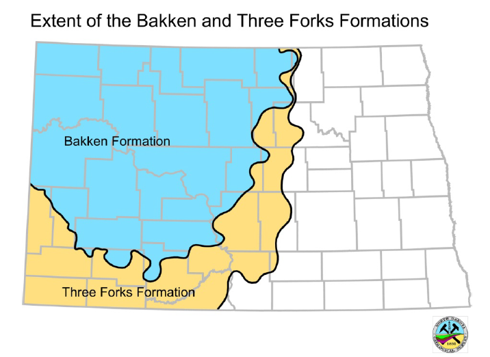
It is noted that the Bakken Petroleum System of the Williston Basin (North Dakota and Montana, USA) consists of the Late Devonian to Early Mississippian Bakken Formation, the underlying Three Forks Formation, and the overlying lower Lodgepole Formation (Early Mississippian). The Bakken Formation is stated to compose of four distinct informal members which include the Pronghom member formerly defined as Sanish sand, the lower shale member, the middle Bakken member, and the Upper shale Member [22]. It was confirmed that the primary reservoir targets are the low porosity and low permeability members of the middle Bakken and upper Three Forks with continued exploration into the middle and lower intervals of the Three Forks Formation and the Pronghorn member [23, 24].
Oil production in the Bakken and Three Forks Formations began in the early 1950s at Antelope Field (North Dakota). Oil drilling was shifted to the Billings Nose area (North Dakota), where the upper Bakken shale was exploited. It was recorded that the first horizontal well was drilled in this region in 1987. As drilling continues in the Three Forks Formation, it has expanded north and south along the main structure of the Nesson anticline, as well as east into the Parshall Field region and the central Williston Basin (North Dakota) [23, 25, 26, 27] (Figure 1).
The Bakken and Three Forks Formations were evaluated by the U.S. Geological Survey (USGS) in 2013, resulting in unexplored, technically recoverable mean resource estimates of 3.65 billion barrels of oil (BBO) for Bakken Formation and 3.73 BBO for the Three Forks Formation (total mean resource estimate of 7.38 BBO; Gaswirth and Marra [23]). IHS Markit® [27] reports that more than 6,400 wells have been drilled in the Bakken Formation since the 2013 assessment. It is also worth mentioning that about 4,100 wells have been drilled in the underlying Three Forks Formation and an estimated 4 billion barrels of oil have been produced from the Bakken and Three Forks Formations [27] (Figure 2).
It was stated that since 2010, the production in the Bakken has generally increased, with various declines beginning in 2014 due to a drop in oil prices and in mid-2020 due to the decrease in demand during the ongoing COVID-19 pandemic. Also, due to drop in well completions, production growth may not rebound until 2022 [29]. Overall, oil production has remained high, and North Dakota continues to be the second largest oil producing state in the country.
![Figure 1: The Bakken and Three Forks Formation Assessment Units (AUs) Map [28].](/fulltextimages/9636/fig_1.png)
Methodology
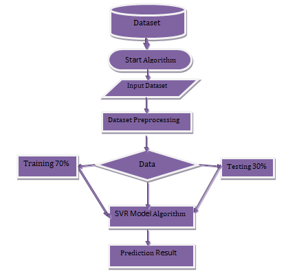
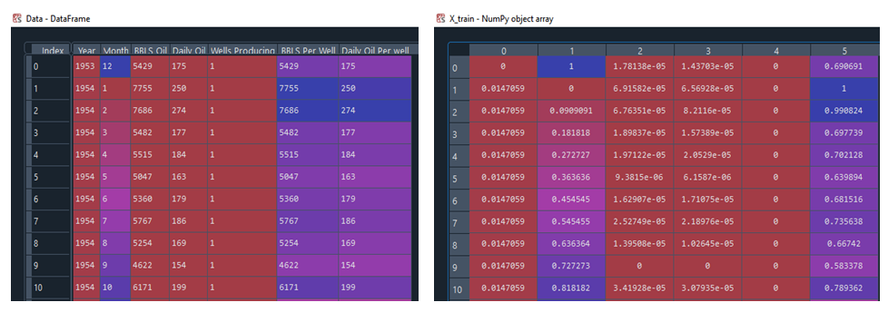
The Support vector Regression was used in Python to predict the Daily Oil per well of the Bakken and Three Forks Formations. The result obtained was validated using the Orange-Linear regression algorithm Software. The dataset obtained from North Dakota Industrial Commission (NDIC) has 817 total instances with both independent variables and dependent value (Figures 3 & 4).
Support vector machine (SVM) is a learning machine that can be used for both classification and regression problems [9]. Support vector regression (SVR) is becoming increasingly popular as a method of curve fitting in linear and non-linear regression problems. Based on the principles of support vectors, SVR operates in the areas of SVM where data points are analyzed in n-dimensional feature space along the hyperplane.
To predict continuous output, hyperplanes are used as decision boundaries. Kernel was employed as the mathematical function that transforms data input into the desired form.
The generalized equation for hyperplane may be represented as:
y = wX + b (1)
where w is weights and b are the intercept at X = 0.
The SVR regression model is imported from SVM class of sklearn python library.
The regressor is fit on the training dataset. The model parameters as chosen here for analysis is shown below.
SVMClass = svm.SVR(kernel=’rbf’, C= 2777.777777777778 , gamma= 0.6444444444444445 ,epsilon= 0.17777777777777778 ). The margin of tolerance is represented by epsilon ε.
In this study, the Support Vector Machine with RBF kernels is used.
In general, the class predictor trained by SVM has the form [equation]
(2) but in the case of a linear kernel K(x, z) = xTz this can be rewritten as [equation]
(3) where the vector of weights w = (w1,...,wd) can be computed and accessed directly. Geometrically, the predictor utilizes a hyperplane to differentiate the positive from the negative instances, and w is the normal to the hyperplane.
Data Pre-Processing
The dataset was processed after importing the data. The aim is to transform the raw data into an understandable format for analysis by a machine learning model. To improve the quality of the result, the dataset was preprocessed in the following order. Data Cleaning: Filling the missing values, smooth noisy data, identify or remove outliers, and resolve inconsistencies. Data Integration: At this point, integration of multiple databases, data cubes, or files was carried out. Data Transformation: This stage involves the normalization and aggregation of the obtained dataset. Thus, the process of converting data to a different format, structure, or value. Normalization is the Data transformation method used for scaling in this project. Data Reduction: The data volume was reduced but the same or similar analytical results were also obtained. Data discretization: The numerical and categorical data at this point was also reduced. In this project three different packages (Microsoft Excel, Python, and Orange) were utilized to obtain the desired accurate results. Data preprocessing for this project is very important because it made the quality of the raw data to be improved.
Visualization of Data
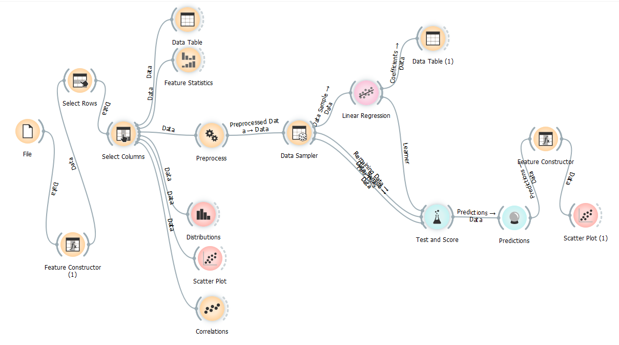
The visual representation of data and information is called data visualization. Data visualization tools utilize visual elements such as charts, graphs, maps, etc. to provide an accessible way to see and understand trends, outliers, and patterns in data (Figure 5).
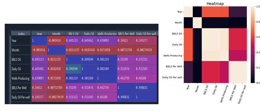
Heat Map
Correlation heat map explains a rough correlation between one parameter with another parameter. The value is between -1 and +1, where +1 shows a perfect correlation between two investigated parameters (Figure 6).
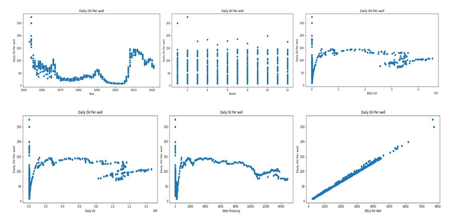
Scatter Plots
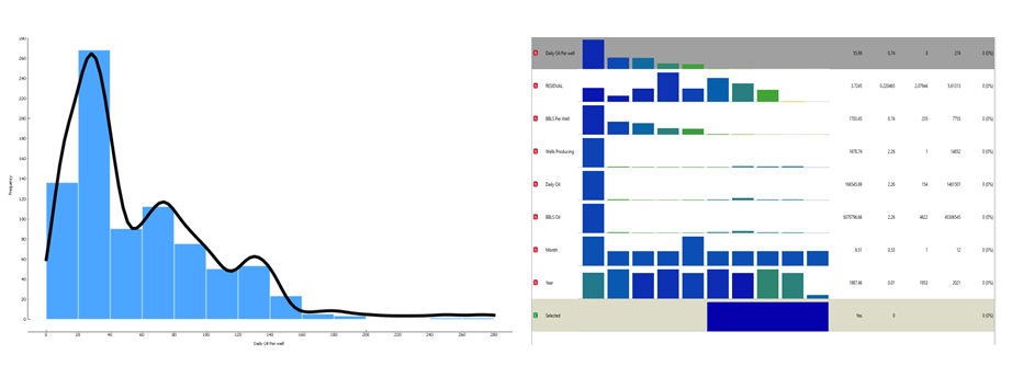
Dataset Distribution
Data Splitting
For the algorithm to interpret the relationship between the dependent and independent variables, there is a need to train the machine learning algorithms. After the training was completed, the trained algorithm was evaluated using a different set of data to test its accuracy. The 817 total instances were partitioned into 70% (571) training set and 30% (246) testing set.
The Daily oil per well generated was compared with the actual Daily oil per well. A support vector regression was performed to improve the quality of the selected algorithm and match the actual Daily oil per well.
The algorithms used for Prediction are Python-Support Vector Regression and Orange-Linear Regression.
Support Vector Regression and Linear Regression
Support vector regression is an algorithm that predicts discrete values through supervised learning. SVR works by finding the hyperplane with the most points, which is the best fit line. In the development of this model in Python, the following steps were followed. First, all the required data was imported and visualized. Featured engineering was then employed and this basically uses the main knowledge to the needed features from the primary data using data mining techniques. The train_test_split was imported from sklearn library which I used to split the dataset into training and testing data. After I succeeded with the splitting of the dataset, I imported the SVR from sklearn.svm library and the model is fitted over the training dataset. In this project, I used the RBF Kernel which gave an accurate prediction.
In linear regression, the relationship between a scalar response and one or several explanatory variables (dependent and independent variables) is modeled linearly.
0 1 ( ) f x b b x = + (4)
To fit a predictive model to observed data sets of response and explanatory variables, linear regression is used. It can be said that when the model has been developed, predictions can be made of the response by using the fitted model when additional explanatory variables are collected without a response value.
Model Evaluation
This project was evaluated using the R2, RMSE, MAE and MSE to measure the performance of the developed model.
R-Squared (R2) is simply a measure of a goodness of fit for Linear regression model. It shows the strength of the relationship between the model developed and the dependent variable on a convenient 0-1 scale.
SSregression R Squared SStotal − = (5)
Where: SSregression is the sum of squares due to regression and SStotal is the total sum of squares.
Root Mean Square Error (RMSE) is defined as the prediction errors (residuals). Which is a measure of how far from the regression line data points.
2 ( ) RMSE f O = − (6) Where f is the forecasts (expected values or unknown results), and 0 is the observed values (known results).
Mean Absolute Error (MAE) is defined as a measure of errors between paired observations expressing the same phenomenon.
i MAE yi xi n = = − ∑ (7)
1 / n Where yi= prediction, xi= true value, n= total number of data points Mean Squared Error (MSE) measures the average of the squares of the errors.
i MSE n yi y i = = ′ − ∑ (8)
( ) 2
1 1/ n Where n=number of data points, yi=observed values and =predicted values
Results
Python-Support Vector Regression
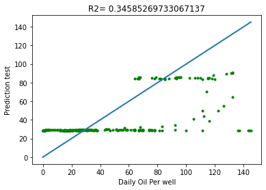
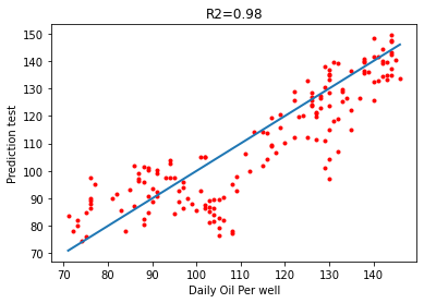
The Daily oil production per well prediction was achieved after undergoing series of processes. Started with the collection of Dataset, Imported the dataset into the Python workspace, Preprocessed the data making sure that it’s clean for the task. Transformation was also done by normalizing it. The Support Vector Regression (SVR) was built with Kernel rbf choice of selection of the regression, values of C, gamma and epsilon were added. 817 total instances were collected, 70% (571) was used to train the model while 30% (246) was used to test the trained model. Plots of the independent variables with dependent variables were modeled to show the relationship of these variables. The Train set MSE is 914.88 and Test set MSE is 931.93. The Test set R2 is 0.35 as shown in the Figure 9 below.
The support vector regression gives the following values in the table below
| MODEL | RMSE | MAE | R2 |
|---|---|---|---|
| SVR Model | 16.593 | 10.593 | 0.98 |
Table 1: SVR Statistical Evaluation Criteria.
The performance of the model in Table 1 above showed a great improvement with the values of the statistical evaluation criteria used. The R2 is 0.98 from the low value of 0.35, the MAE became 10.593 and RMSE is 16.593. The performance of this SVR model indicate that this developed model can be used to predict the Daily oil production per well accurately with the supervised algorithm. The relationship of the predicted test versus the Daily oil per well is shown in the Figure 10 below with R2 of 0.98.
Orange-Linear Regression
This Table 2 shows the values of the Daily oil per well predicted by the regression model. For a 70 bbls, the model predicted 70.9587 bbls. For 71 bbls, the predicted Linear regression value is 69.1767 bbls. With the predicted values obtained, this model can be utilized to accurately predict the Daily oil per well for an oil production forecast for a given formation.
| Daily Oil for well | Selected | Linear Regression | Fold | |
|---|---|---|---|---|
| 70 | Yes | 70.9587 | 1 | |
| 71 | Yes | 69.1767 | 1 | |
| 82 | Yes | 82.769 | 1 | |
| 73 | Yes | 75.2406 | 1 | |
| T7 | Yes | 71.2672 | 1 | |
| 78 | Yes | 79.8371 | 1 | |
| 58 | Yes | 57.5714 | 1 | |
| 39 | Yes | 39.8841 | 1 | |
| 60 | Yes | 59.089 | 1 | |
| 68 | Yes | 69.6739 | 1 | |
| 74 | Yes | 75.m | 1 | |
| 75 | Yes | 73.343 | 1 | |
| 68 | Yes | 68.7648 | 1 | |
| MODEL | MSE | RMSE | MAE | R2 |
| Regression with cross validation of 10 folds | 2.826 | 1.681 | 1.045 | 0.998 |
| Test on test data | 4.468 | 2.114 | 1.640 | 0.980 |
Table 2: Actual versus predicted values.
This model can be applied in several oil and gas prediction and forecasting analysis. With results obtained in Figure 10 and Table 2, It clearly shows that the developed algorithm can be effectively used in almost all fields of study if the independent variables are well known and stated. As well as the unknown dependent variable is related to the independent variables.
As shown in Table 3 above, the regression with a cross validation of 10 folds for the 70% train dataset and 30 % test dataset shows MSE value of 2.826, RMSE of 1.681, MAE of 1.045 and R2 value of 0.998. The R2 value that is approximately equal to 1 proves that the developed machine model is a good tool for accurate prediction of the Daily oil produced by a well. The criteria (MSE, RMSE, MAE & R2) used for the evaluation are dimensionless.
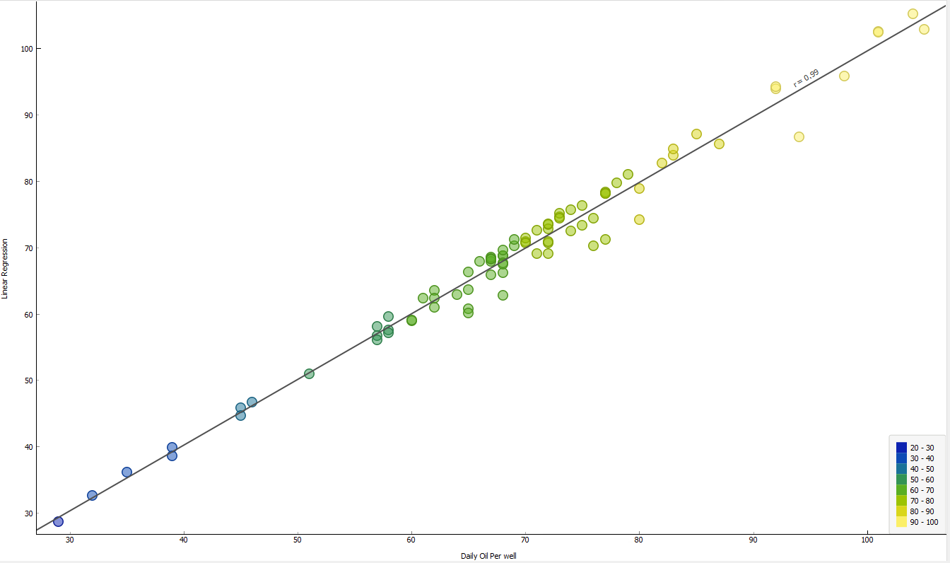
Figure 11 above shows the relationship between Regression model developed versus Daily oil production per well with R2 value of 0.99. Which clearly confirms a great performance of the model. The result obtained validates the predicted value obtained using the Support Vector Regression.
Conclusion
It was shown with these models developed that the Daily Oil production per well can be accurately predicted as the dependent variable using the independent variables (Year, Month, BBLs oil, Daily Oil, Wells producing, and BBLs per well) by applying the knowledge of Data mining in petroleum Engineering gained in the lectures and tutorials. The model development started by collecting the dataset from the North Dakota Industrial Commission (NDIC). Followed by Preprocessing (Cleaning, Integration, Transformation, Reduction and Discretization) of the dataset. Data splitting which was basically to partition the dataset into 70% training and 30% testing. Normalization of the dataset was done by using the MinMax scaler. The Support Vector regression was tested using the 70% trained model partitioned.
The result obtained at first didn’t match the trained dataset well enough until the SVR model was developed with values of C, gamma and Epsilon clearly stated. The values for R2 became 0.99 from its initial value of 0.35. Likewise, the values of RMSE reduced to 16.593 and MAE reduced to 10.593. This project used both the Python-Support vector regression and Orange-Linear regression algorithm to predict the Daily oil production per well by Bakken and Three Forks formations. This machine learning algorithm was able to accurately forecast the daily oil production per well from the given datasets. Comparing the results obtained from both software, it is seen that the values obtained from the Orange-Linear regression show better performance which also validates the values obtained from the Python Support Vector Regression.
Application of this algorithm is not limited to just research; it can be generally used for all forecasting and prediction related problems in all fields given that there is a relationship between the dependent variable and the independent variables.
References
-
Fisher RA (1936) The use of multiple measurements in taxonomic problems. Ann Eugenics 7(2): 179-188.
-
Rosenblatt F (1962) Principles of Neurodynamics: Perceptrons and the Theory of Brain Mechanisms. Spartan Books, Washington DC.
-
Rumelhart DE, Hinton GE, Williams RJ (1986) Learning internal representations by backpropagating errors. Nature 323: 533-536.
-
Rumelhart DE, Hinton GE, Williams RJ (1986) Learning internal representations by error propagation. In: James L, et al. (Eds.), Parallel Distributed Processing. University of Toronto, Canada, pp: 318-362.
-
Parker DB (1985) Learning-Logic: Casting the Cortex of the Human Brain in Silicon. Technical Report TR- 47, Center for Computational Research in Economics and Management Science, Massachusetts Institute of Technology, Cambridge, USA.
-
LeCun Y (1985) A learning procedure for asymmetric threshold network. Proceedings of Cognitive, Paris, France, 85.
-
Ali JK (1994) Neural Networks: A New Tool for the Petroleum Industry. European Petroleum Computer Conference, Aberdeen, UK.
-
Mohaghegh S, Ameri S (1994) Artificial Neural Network as a Valuable Tool for Petroleum Engineers. Society of Petroleum Engineers, Paper SPE 29220.
-
Cortes C, Vapnik VN (1995) Support Vector Networks. Machine Learning 20(3): 273-297.
-
Simon T, Daphne K (2001) Support Vector Machine Active Learning with Applications to Text Classification. Journal of Machine Learning Research, pp: 45-66.
-
Basak D, Pal S, Patranabis DC (2007) Support vector regression. Neural Inf Process Lett Rev 11: 203-224.
-
Laura A, Rouslan AM (2008) Support Vector Machines (SVM) as a technique for solvency analysis. DIW Discussion Papers, No. 811, Deutsches Institut für Wirtschaftsforschung (DIW), Berlin.
-
Anifowose F, Abdulraheem A (2010) Prediction of Porosity and Permeability of Oil and Gas Reservoirs using Hybrid Computational Intelligence Models. SPE North Africa Technical Conference and Exhibition, Cairo, Egypt.
-
Anifowose F, Abdulraheem A (2010) A Fusion of Functional Networks and Type-2 Fuzzy Logic for the Characterization of Oil and Gas Reservoirs. International Conference on Electronics and Information Engineering, Kyoto, Japan.
-
Helmy T, Anifowose F (2010) Hybrid Computational Intelligence Models for Porosity and Permeability Prediction of Petroleum Reservoirs, International Journal of Computational Intelligence and Applications (IJCIA) 9(4): 313-337.
-
Ho CH, Lin CJ (2012) Large-scale Linear Support Vector Regression. Journal of Machine Learning Research 13: 3323-3348.
-
Zhang Y (2012) Support Vector Machine Classification Algorithm and Its Application. In: Liu C, et al. (Eds.), Information Computing and Applications. Springer, Berlin, Heidelberg, pp: 179-186.
-
Falode OA, Udomboso C, Ebere F (2016) Prediction of Oilfield Scale formation Using Artificial Neural Network (ANN). Advances in Research 7(6): 1-13.
-
Wang H, Xiong J, Yao Z, Lin M, Ren J, et al. (2017) Research Survey on Support Vector Machine. Proceedings of 10th EAI International Conference on Mobile Multimedia Communications, Chongqing, People’s Republic of China, pp: 95-103.
-
Ruidong W, Bing L, Jiafeng F, Mingzhu X, Ping (2019) Research and Implementation of ε-SVR Training Method Based on FPGA. Electronics 8(9): 919.
-
Su X, He X, Zhang G, Chen Y, Li K (2022) Research on SVR Water Quality Prediction Model Based on Improved Sparrow Search Algorithm. Comput Intell Neurosci 2022: 1-23.
-
Fever JAL, Fever LRD, Nordeng SH (2011) Revised nomenclature for the Bakken Formation (Mississippian- Devonian), North Dakota. Rocky Mountain Association of Geologists, pp: 11-26.
-
Gaswirth SB, Marra KR (2015) U.S. Geological Survey 2013 assessment of undiscovered resources in the Bakken and Three Forks Formations of the U.S. Williston Basin Province. AAPG Bulletin 99(4): 639-660.
-
Sonnenberg SA (2017) Sequence Stratigraphy of the Bakken and Three Forks Formations, Williston Basin, USA. In: Hart B, et al. (Eds.) Sequence Stratigraphy: The Future Defined. SEPM Gulf Coast Section Publications, Williston Basin.
-
Sonnenberg SA, Pramudito A (2009) Petroleum geology of the giant Elm Coulee field, Williston Basin. AAPG Bulletin 93(9): 1127-1153.
-
Nesheim T (2019) Examination of downward hydrocarbon charge within the Bakken-Three Forks petroleum system-Williston Basin, North America. Marine and Petroleum Geology 104: 346-360.
-
IHS Markit (2021) US well history and production database. Enerdeq™, Englewood Cliffs, USA.
-
Marra K (1953) Bakken and Three Forks Formations Williston Basin North Dakota and Montana. US Geological Survey, Central Energy Resources Science Center, Denver, Colorado, USA
-
Tobben S (2020) North Dakota regulator sees Bakken shale growth stalled until 2022.
- Nigeria’s Vulnerability in the Face of Global Energy Policy
- A Simulation Study of Investigation of Optimum Oil Production Performance by Applying Various Gas Injection Methods in Oil Reservoir
- Characterization of Permo-Triassic Reservoirs through Thermal Maturity Assessment of Westphalian Source Rocks in the Cheshire Basin
- Influence of Microwax on the Rheological and Thermal Behaviour of a Wax Crude Oil
- Real-Time Monitoring and Performance Optimization of Steam Injection in Heavy Oil Reservoirs Using Fiber Optic Sensing and Integrated Predictive Simulation Models
- Rapid On-Site Determination of the Total Petroleum Hydrocarbon Content of Soils by Handheld Fourier Transform Near-Infrared Spectroscopy: Development of a Global, Site- and Scanner- Independent Calibration Model