Thermochemical Advanced Oxidation Process by DiCTT for the Degradation/Mineralization of Effluents Phenolics with Optimization using Response Surface Methodology and Artificial Neural Networks Modelling
The actual work evaluated the effect of initial phenol concentration (CPh0) of 500, 1000 and 1500 mg.L-1, the molar stoichiometric ratio of Phenol/Hydrogen peroxide (RP/H) of 25, 50 and 75 % and time (t) of 30, 90 and 150 min on the oxidation of phenolic effluents by called Direct Contact Thermal Treatment (DiCTT). This process provides a novel means to induce degradation and mineralization of organic pollutants in water. The experimental studies were carried out at semi-industrial plant. The organic pollutant was degraded with a conversion higher than 99% and a Total Organic Carbon (TOC) mineralization exceeding 40%, to a (RP/H) of 75%, independent of the CPh0, that was identified as the optimal condition by thermochemical process. The initial phenol concentration was quantified and identified by the High Performance Liquid Chromatography (HPLC) technique followed by statistical design tools to optimization using Response Surface Methodology (RSM) and an analytical mathematical modelling via Artificial Neural Networks (ANNs). The results also showed the dynamic concentration evolution of the intermediates formed (catechol, hydroquinone and para-benzoquinone). Artificial Neural Networks were applied to model the step experimental of Phenol Degradation (PD) and Total Organic Carbon (TOC) conversion by DiCTT thermochemical process. For the ANN modelling, “statistic 8.0” software was used with a Multi-Layer Perceptron (MLP) feed-forward networks by input-output data using a back-propagation algorithm. The correlation coefficients R2 between the network predictions and the experimental results were in the range of 0.95–0.99.
Graphical Abstract
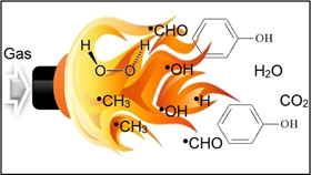
modelling via Artificial Neural Networks (ANNs). The results also showed the dynamic concentration evolution of the intermediates formed (catechol, hydroquinone and para-benzoquinone). Artificial Neural Networks were applied to model the step experimental of Phenol Degradation (PD) and Total Organic Carbon (TOC) conversion by DiCTT thermochemical process. For the ANN modelling, “statistic 8.0” software was used with a Multi-Layer Perceptron (MLP) feed-forward networks by input-output data using a back-propagation algorithm. The correlation coefficients R2 between the network predictions and the experimental results were in the range of 0.95–0.99.
Keywords: Phenol; Thermochemical Oxidation; AOPs; DiCTT; ANNs
Introduction
The water is essential for life, being an important natural resource, both for a biochemical component of living beings, and through the life of various species, such as: vegetables and animals. Thus, the treatment, and management of chemical pollutants in the environment is a matter of extreme relevance for environmental sustainability. Therefore, the efficient removal of Persistent Organic Pollutants (POPs) from wastewater streams is severely important, due to their possible mutagenic and carcinogenic characteristics, as well as their acute and chronic consequence on human health mainly [1].
Phenol is considered one of the most toxic aromatic and refractory organic compounds found in wastewater released by various industries [2]. Wastewaters of industrial plants, often exhibit high levels of organic compounds, which are harmful to human health and the environment [3]. Phenol and BTEX (benzene, toluene, ethylbenzene and xylenes) are also added to the class of organic substances analysed as hazardous chemicals [4]. The great relevance in industrial and municipal treatment methods is the removal of contaminants present in wastewater through chemical, physical and biological processes [5]. The main sources of organic pollutants are oil refineries and petrochemical plants, coke gasifiers, pulp and paper production, pharmaceuticals, the food industry and plants that process minerals, plastics, metals and organic chemicals [6].
The primary impact of these industries on the environment is the generation of highly polluted wastewater. The organic pollutants most detected in those wastes are phenol: C6H5OH, 2-chlorophenol: C6H5ClO, 2,4-di-chlorophenol: C6H4Cl2O, 2,4,6-tri-chlorophenol: C6H2Cl3OH/C6H3Cl3O, 2-nitrophenol: C6H5NO3, 4-nitrophenol: C6H5NO3, 2,4-di- nitrophenol: C6H4N2O5, 2-metilphenol: C7H8O, 3-metilphenol: C7H8O, 4-dimetilphenol: C8H10O and 4-aminophenol: C6H7NO [7]. There are several physicochemical and biodegradation methods that have been employed to treat industrial effluents containing phenolic and refractory organic compounds, such as ozonization, adsorption, photocatalysis, use of membranes and enzymatic treatment [8]. Phenol removal has also been employed from an osmotic membrane bioreactor for the treatment of effluents [9].
Phenols have antiseptic properties that are explained by bactericidal action and are currently used in phenolic compounds such as espadol, creolin, and lisol, which are disinfectants due to their mechanism of coagulating microorganism proteins. Phenol is also used in the production of polymers (bakelite), pyric acid and its derivatives (explosives and burn medications), indicators (phenolphthalein), dyes, resins and salicylic acid [10]. However, phenolic compounds are harmful to human health and can cause necrosis, digestive problems, liver and kidney damage [11]. Phenols cause toxicity and are carcinogenic, so these compounds can provide bad odor and contaminate water, even in low concentration [12]. The presence of phenolic contaminants in sublethal doses affects the nervous and circulatory system, with reduced growth of blood cells [13]. Phenol vapors when inhaled through the airways, causes dyspnea (difficulty breathing), coughing and are quite corrosive to tissues. When exposure to concentrations of these compounds are high, it causes tachypnea, bronchopneumonia, bronchitis, pulmonary edema, and respiratory arrest. In the central nervous system arises initially excitement, and soon after, depression, which causes convulsions and unconsciousness. Contact with the skin and mucous membranes produces irritation, burns, inflammation and discoloration. It can also cause from an erythema to necrosis and gangrene in tissues, depending on the time of contact and the concentration of solutions [14]. When present in drinking water, phenols can cause serious public health problems and can also cause the death of fish, even at concentrations in the range of 1 mg. L-1. At concentrations of less than 1 mg. L-1, are also toxic to other biological species and destroy the aquatic environment [15]. Phenol has an identifiable taste in water, even at low concentrations of 0.002 mg.L-1. From an exposure time of around 4 days and concentrations ranging between 10 and 100 mg.L-1, these compounds are lethal to many aquatic lives. Phenol can be detected at concentrations of only 40 μg.L-1 in the air and about 1-8 mg.L-1 in water [16].
The toxicity of these compounds in water has had quite relevance due to their concentrations that at mg.L-1 levels, may affect the aquatic environment [17]. Thus, the various aromatic compounds present should be constantly identified and monitored. Therefore, there is a need to restore contaminated areas with these organic compounds and avoid further contamination of the environment [18]. The solution of such task requires a broad understanding of the chemicals and biological concepts of the potential contaminants [19].
In recent decades, several demands were suggested for the definition of strategies in order to improve existing processes and develop clean technologies to degrade a greater amount of toxic and polluting substances, which were generated by either the available methods process, such as, industrial wastes or municipal wastes [20]. Thus, the removal of organic pollutants from the environment has been a major technological challenge, because, in many times, conventional treatment technologies are not able to solve the problem efficiently. For this reason, the search for these effective technologies has grown so much to be destroyed [21]. The legislation through resolution No. 430, published on May 13, 2011, of the National Council for the Environment (CONAMA) establishes the maximum value for the presence of organic substances in effluents, such as chloroform, dichloroetene, carbon tetrachloride and trichloroetene, the limit of 1 mg. L-1, and for the presence of total phenols (substances that react with 4-aminoantipyrine) the maximum limit of 0.5 mg.L-1 [22].
There are several processes used in the treatment of industrial liquid effluents that can be divided into three main groups: biological, chemical and physical. A combination of these processes is generally used. The efficiency of the biological process in destroying organic substances can reach 97%. However, certain factors such as organic matter concentration and temperature can adversely affect the efficiency of such processes [23]. An alternative to biological treatment is incineration, however its use is limited when the Chemical Oxygen Demand (COD) is low, below 200 g.L-1, due to the amount of energy required [24]. Physical processes have disadvantages in relation to selectivity in the treatment of liquid effluents and require storage and disposal of removed contaminants. Chemical processes are often limited with respect to the volume of liquid to be treated [25]. Currently, alternative methods were analyzed for the degradation stage of domestic and industrial liquid effluents containing organic compounds, such as catalytic oxidation, photo-oxidation and electrochemical oxidation, ultrafiltration and combined methods. Another auxiliary method for removal is the adsorption technique, which depends on the adsorptive materials used [26].
In recent years, between the various methods of wastewaters treatment containing toxic organic substances, Advanced Oxidation Processes (AOPs) have been studied as an alternative technology for the treatment of toxic organic effluents [27]. This AOPs has been largely used in pre- treatment on olive oil mill effluent using physicochemical, Fenton and Fenton-like [28]. This method by AOPs has also been applied through the use of ozone (O3, O3/H2O2, O3/UV and O3/UV/H2O2) for the treatment of textile effluents [29]. These processes have as main advantages the ability to degrade a toxic substance or convert it into a biodegradable form, due to the generation of hydroxyl radicals (•OH), species capable of attacking the majority of organic molecules [30]. Phenol catalytic oxidation has been applied with a heterogeneous Cu(II) onto Chitosan and poly(4-vinylpyridine) (PVP) catalysts in a reactor for municipal wastewater treatment using air and H2O2 as oxidants [31]. The stage of phenol photodegradation and formation of organic intermediates and •OH radicals were studied by UV/TiO2 and Vis/N, C-TiO2 processes [32]. Catalytic phenol degradation in sonolysis was studied by coal ash and H2O2/O3 as oxidants [33]. The toxicity of phenol solutions was analysed using oxidative systems such as H2O2/UV and H2O2/Fe [34]. The oxidation of triclosan by ferrate (Fe (VI)) was investigated to determine intermediates formed and evaluate the toxicity variations during this oxidation step during this oxidation step [35]. AOPs has also been applied through the procedure of sulphate radical by photooxidation (UV/PMS/PS), sonooxidation (US/PMS/PS) and sono-photooxidation (US/ UV/PMS/PS) with peroxymonosulfate (PMS) and persulfate (PS) as oxidants for simulated dyehouse effluent treatment [36]. AOPs are attractive technologies including photolysis, photocatalysis and Fenton oxidation for the degradation of Polychlorinated dibenzo-p-dioxins and dibenzofurans (PCDD/Fs) in wastewater. These compounds are considered a family of persistent organic pollutants (POP) because of their potential toxicity when discarded in the environment [37]. The UV photolysis with hydrogen peroxide (UV/H2O2) are effective treatments for phenolic compounds because of the reactions that occur during the effluent degradation stage, which includes mechanisms of intermediate reactions with •OH radicals [38]. AOPs has also been studied based on pre-magnetization Fe0 for wastewater treatment because these compounds are capable of destroying recalcitrant organic substances in other less toxic products by the use of radicals (•OH and SO4 -) [39].
An unconventional AOP named Direct Contact Thermal Treatment (DiCTT) was developed [40]. The DiCTT process presents operational and capital costs 2.5 fold lower than those of Wet Air Oxidation (WAO) and 4.1 fold lower than those of Electric Plasma Oxidation (EPO). The experimental set-up, a vertical reactor, is compact and allows easy operation. This technique is appropriate for off-shore oil drilling platforms, where natural gas is available and space is limited, reported by Benali, et al. [41], and it is based on the thermochemical oxidation of organic compounds dissolved in an aqueous medium. Free radicals such as •OH, •H, •CH3 and •CHO are generated from the combustion of natural gas (methane) according to the reaction mechanism defined by Benali and Guy [42] described in the following Equation (1):
A →
- B +
- C
- B + O2 → D +
- E
- E + A →
- B + H2O
- E + A →
- F +
- E + 3/2 H2 (1) Where: A= (CH4-Methane);
- B= (
- CH3-Methyl Radical);
- C= (
- H-Hidrogen Radical);
- E= (
- OH-Hidroxyl Radical); D= (CH2O-Methanal); O2 = Molecular Oxygen; H2O = Water;
- F= (
- CH- Methylidyne Radical); H2 = Molecular Hidrogen.
Statistical techniques commonly referred to as Response Surface Methodology (RSM) are powerful experimental design tools that have been used to optimise and evaluate the performance of difficult systems [43]. As well as Artificial Neural Networks (ANNs) also are strategic able tools for modelling and optimisation complex [44], non- linear methods with uncertain dynamic models [45]. Thus, ANNs have been used to the processes, such as biological and physicochemical wastewater treatment, respectively. However, few studies have been published in the literature showing the applications of ANN in AOPs in the treatment of organic effluents containing phenol [46]. Thus, ANNs must be trained, tested and validated for a data set appropriate to model the neural network to resolve the complexity of obtaining phenomenological models.
This research presents showed as novelty the extent of experimental tests, which analyzed the optimal operational conditions by the thermochemical process for complete phenol degradation and TOC conversion, regardless of the initial concentrations of phenol. The effect of the three factors CPh0, RP/H, and t were investigated. The input variables were initial phenol concentration, CPh0, of 500, 1000 and 1500 mg L-1, the molar stoichiometric ratio of Phenol/Hydrogen peroxide, RP/H, of 25, 50 and 75% and collections times (t) of 30, 90 and 150 min. The liquid phase flow rate, QL, was 170 L h-1, burner power dissipation, P, of 38.6 kW, air excess, E, of 10% and a recycle rate of gaseous thermal wastes, QRG, of 100%. Optimal conditions were identified for complete phenol degradation (>99%) and TOC conversion (>40%), to R of 75%, regardless of CPh0, and t of 150 min, being the best operational time studied to date by the optimized conditions of the DiCTT process. This study is the type of process modeling with optimization using RSM and ANNs for the Phenol Degradation (PD) and Total Organic Carbon (TOC) conversion by DiCTT thermochemical process. Thus, the method of modelling, i.e., RSM, was used to determine the relationship between input and output variables for the experimental complete factorial design type with factorial k, 23, includes duplicate in each sample and six repetitions at the Centre Point (CP), totalling 22 runs and collection times, t, of 30, 90 and 150 min. The two methods of modelling was employed to evaluate the influence of the key variables on the process efficiency and at the steps of phenol oxidation and formation of their aromatic by-products, mainly, hydroquinone and catechol, and mineralization of them into carbon dioxide and water. Therefore, this method uses the smallest possible quantity of data and analyses all sets of data with the goal of optimising the operating conditions for the degradation/mineralization of phenol and its by-products by the DiCTT process. Thus, the output variables were the PD and TOC conversion. The importance of each input variable on the discrepancy of the output response was determined and compared with the results obtained by RSM and ANNs. The phenol concentration and mineralization content were obtained by High Performance Liquid Chromatography (HPLC) and Total Organic Carbon (TOC) Analysis, respectively. These results were achieved using statistic software version 8.0.
Materials and Methods
Reagents
The experiments were performed in a reactor using a prepared phenol solution (99% PA, Dinâmica) and oxygenated water, H2O2, analytical grade (35% PA, Vetec). The methanol was used, UV/HPLC (99.9% PA, Vetec) in the chromatographic analysis, and phosphoric acid, H3PO4 (25% PA, Vetec) was used in the TOC analysis.
Pilot Plant and Experimental Procedures
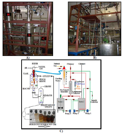
Figure 1A & B shows the photograph of the installation of the DiCTT pilot unit. Figure 1C shows a schematic representation of the pilot plant used in the experiments that was composed of a vertical, stainless-steel reactor and a gas–liquid separator. The phenol solution was prepared in Tank 1 with a 250-L volume by heating the water to almost 70°C for an hour and a half; the synthetic effluent was transferred from Tank 2 and after was injected into the reactor tangentially to produce a liquid helical stream on its inner walls. The combustion gases were vented to the atmosphere through a chimney; a fraction of recycled combustion gases, of the total flow rate QRG, was immediately injected into Tank 2 by adjusting an open valve to heat the solution in the recirculation tank, Tank 2, more rapidly and to dissolve a fraction of the residual oxygen from combustion into the reaction liquid, thereby inducing the thermochemical oxidation of the phenolic compounds. For each assay, samples of approximately 250 mL of solution were collected in duplicate, at the different points and regular times, in dark plastic bottles and were refrigerated. A 250 mL sample of treated water without phenol was also collected to serve as a blank for the phenol solutions. The molar ratio fraction of phenol/hydrogen peroxide, RP/H, was introduced into the recirculation tank, Tank 2, to initiate the phenol oxidation in the aqueous phase [47].
Analytical Methods
High-performance liquid chromatography (HPLC): The concentrations of phenol, catechol and hydroquinone were monitored using High-Performance Liquid Chromatography (HPLC) Shimadzu, model LC-20AT, with integrated data acquisition using a UV detector and a CLC-ODS column M/C- 18 that was 250 mm in length and 4.6 mm in diameter, also from Shimadzu. An isocratic elution mode was used under the following conditions: oven temperature of 35°C; flow rate of the mobile phase, 0.75 mL min-1; injection volume of 20 μL; mobile phase consisting of 10% methanol and 90% phosphoric acid/deionised water with pH adjusted to 2.2; and UV detector wavelength, 270 nm to detect phenol, catechol and hydroquinone [47].
Total organic carbon (TOC): The Total Organic Carbon (TOC) content was measured using a TOC analyser, TOC- Vcsh model, Shimadzu, to analyse phenolic mineralisation quantitatively. The TOC is the difference between the Total Carbon (TC) and the Inorganic Carbon (IC) content [48].
Definitions of operation parameters and calculated magnitudes: A molar stoichiometric ratio of 100% for phenol to hydrogen peroxide corresponds to the number of moles of hydrogen peroxide needed to completely convert 1 mole of phenol into carbon dioxide and water in accordance with the reaction stoichiometry described in the following Equation (2):
C6H5OH + 14 H2O2 → 6 CO2 + 17 H2O (2)
Molar ratios other than 100% were calculated proportionally using the reaction stoichiometry in Equation (2).
For each mole of natural gas, methane, which is oxidised in the combustion process, 9.881 moles of air are needed stoichiometrically. Consequently, the excess air (E) in the combustion of natural gas and the respective equivalent ratio (ϕ) can be evaluated using Equation (3) and Equation (4) from the literature reported by Oliveira [49] with a natural gas composition provided by the Companhia Pernambucana de Gás–Brasil (Pernambuco Gas Company–Brazil) [50]:
Q E Q = −
1 1 9.881 AR (3) GN
Q Q φ = (4)
9.881 GN AR Where: QAR denotes the volumetric flow rate of air, and QGN denotes the volumetric flow rate of natural gas. The power dissipated by the burner, P, was calculated using the following Equation (5):
P= QGN.PCM, (5)
Where: PCM denotes the average combustion heat of natural gas, which has a value of 34.740 kJ m-3 [50].
The percent Phenol Degradation (PD) was calculated using the following Equation (6):
− − =
. . . .100 . , o v
Q C Q C F C PD Q C
L Ph L Ph G Ph
(6) L Ph o Where: QL denotes the volumetric liquid flow rate, CPh0 denotes the initial phenol concentration, CPh denotes the phenol concentration at a given time, FG denotes the mass flow rate of dry air and CPhv denotes the phenol concentration in the condensate at a given time. The percent TOC conversion (TOC) was calculated using the following Equation (7):
− − − = ν ( ) , . TOC TOC . Q TOC . F TOC . Q TOC . Q TOC
0 G L L 100
(7)
0 B L Where: TOC0 denotes the initial total organic carbon concentration, TOC and TOCV denote the total organic carbon and the total organic carbon in the condensate, respectively, at a time point t of the process and TOCB denotes the total organic carbon in the blank.
Experimental Design
Response surface methodology and contour curves: The Response Surface Methodology (RSM) were used for the experimental complete factorial design type with factorial k, 23, includes duplicate in each sample and six repetitions at the Centre Point (CP), totalling 22 runs and sample collection times, t, of 30, 90 and 150 min; as well as optimisation by means of statistical analysis software package, Statistic 8.0. The most popular class of second-order designs was used for Response Surface Methodology (RSM) in the experimental design [51]. The 23 full-factorial is well suited for fitting a quadratic surface, which usually works well for process optimisation [52]. The independent variables, t, of 30, 90 and 150 min; CPh0 of 500, 1000 and 1500 mg L-1; RP/H of 25, 50 and 75%, as well as their experimental ranges, t: –1, 0 and +1; CPh0: –1, 0 and +1; RP/H: –1, 0 and +1 were determined in the experimental design.
Artificial Neural Networks
The Artificial Neural Network (ANN), also called “conexionism”, composed of artificial neurons, had as main purpose, to evaluate certain mathematical functions (usually nonlinear). The ANN was simulated using Statistic 8.0 software with the Neural Network component to predict the Phenol Degradation (PD) and the TOC conversion (TOC). The ANNs are able to solve problems that initially pass in the “network learning” stage from an experimental data set, where input values are provided in order to represent a satisfactory response to the problem. In this work an ANN was created using the following network input factors: the initial phenol concentration (CPh0) of 500, 1000 and 1500 mg.L-1, the molar stoichiometric ratio of Phenol/Hydrogen peroxide (RP/H) of 25, 50 and 75 % and time (t) of 30, 90 and 150 min, where the Phenol Degradation and the TOC conversion was the neural network output. Fifty-seven experimental data points were used to simulate the ANN. Table 1 shows the duplicate data that were achieved for each trial.
In the ANN building was used a Multi-Layer Perceptron (MLP) feed-forward networks by input-output data using a back-propagation algorithm, being this ANN determined by the number of layers, number of neurons (nodes) in each layer, the class of learning algorithms and the functions of transfers. In this step, the number of neurons in the Hidden Layer (HL) and the number of iterations for network calibration were chosen as random variables in the network development. The best choice of the algorithm and transfer function were the primary factors in the conception of the ANN model obtained [53].
In this work, the logistic transfer function (activation) in the hidden layer and in the network output was used for ANN, being the algorithms used to optimise the network the almost Newton method of the type BFGS (Quasi-Newton method with the Hessian approximation proposed by Broyden, Fletcher, Powell and Goldfarb) with differential evolution algorithm. In total, 57 experimental data points were used to generate the ANN, with 80% used for training, 10% for testing and 10% for validation. In total, 5,000 networks were trained. The training was used to adjust the ANN weights and the test to evaluate the neural network configuration.
| Run | t (min) | C Ph0 (mg L-1) | R P/H (%) | PD (%) | TOC (%) | Run | t (min) | C Ph0 (mg L-1) | R P/H (%) | PD (%) | TOC (%) |
|---|---|---|---|---|---|---|---|---|---|---|---|
| 1 | 30 | 500 | 25 | 0 | 0 | 30 | 150 | 1000 | 50 | 98.95 | 26.59 |
| 2 | 90 | 500 | 25 | 52.96 | 16.54 | 31 | 30 | 1000 | 50 | 31.55 | 1.89 |
| 3 | 150 | 500 | 25 | 88.97 | 33.71 | 32 (CP) | 90 | 1000 | 50 | 89.13 | 16.02 |
| 4 | 30 | 500 | 25 | 0 | 0 | 33 | 150 | 1000 | 50 | 99.02 | 27.05 |
| 5 | 90 | 500 | 25 | 53.07 | 16.87 | 34 | 30 | 1000 | 75 | 41.23 | 3.98 |
| 6 | 150 | 500 | 25 | 87 | 33.88 | 35 | 90 | 1000 | 75 | 88.46 | 17.8 |
| 7 | 30 | 500 | 50 | 0 | 0 | 36 | 150 | 1000 | 75 | 99.61 | 38.47 |
| 8 | 90 | 500 | 50 | 83.23 | 16.27 | 37 | 30 | 1000 | 75 | 40.99 | 4 |
| 9 | 150 | 500 | 50 | 98.9 | 37.27 | 38 | 90 | 1000 | 75 | 88.8 | 18.02 |
| 10 | 30 | 500 | 50 | 0 | 0 | 39 | 150 | 1000 | 75 | 99.35 | 38.08 |
| 11 | 90 | 500 | 50 | 84.39 | 15.65 | 40 | 30 | 1500 | 25 | 0 | 0 |
| 12 | 150 | 500 | 50 | 98.47 | 37.58 | 41 | 90 | 1500 | 25 | 40.16 | 3.68 |
| 13 | 30 | 500 | 75 | 0 | 0 | 42 | 150 | 1500 | 25 | 74.91 | 10.03 |
| 14 | 90 | 500 | 75 | 84.92 | 14.86 | 43 | 30 | 1500 | 25 | 0 | 0 |
| 15 | 150 | 500 | 75 | 99.49 | 40.57 | 44 | 90 | 1500 | 25 | 40.37 | 3.91 |
| 16 | 30 | 500 | 75 | 0 | 0 | 45 | 150 | 1500 | 25 | 74.98 | 10.25 |
| 17 | 90 | 500 | 75 | 85.04 | 14.95 | 46 | 30 | 1500 | 50 | 0 | 0 |
| 18 | 150 | 500 | 75 | 99.51 | 40.14 | 47 | 90 | 1500 | 50 | 48.38 | 10 |
| 19 | 30 | 1000 | 25 | 0 | 0 | 48 | 150 | 1500 | 50 | 96.32 | 22.04 |
| 20 | 90 | 1000 | 25 | 52.51 | 8.23 | 49 | 30 | 1500 | 50 | 0 | 0 |
| 21 | 150 | 1000 | 25 | 93.08 | 16.61 | 50 | 90 | 1500 | 50 | 48.72 | 10.79 |
| 22 | 30 | 1000 | 25 | 0 | 0 | 51 | 150 | 1500 | 50 | 96.3 | 21.87 |
| 23 | 90 | 1000 | 25 | 51.99 | 8.47 | 52 | 30 | 1500 | 75 | 0 | 2.03 |
| 24 | 150 | 1000 | 25 | 92.99 | 16.58 | 53 | 90 | 1500 | 75 | 84.95 | 12.98 |
| 25 | 30 | 1000 | 50 | 31.46 | 1.88 | 54 | 150 | 1500 | 75 | 99.1 | 37.8 |
| 26 (CP) | 90 | 1000 | 50 | 88.78 | 15.97 | 55 | 30 | 1500 | 75 | 0 | 1.99 |
| 27 | 150 | 1000 | 50 | 98.44 | 27.03 | 56 | 90 | 1500 | 75 | 83.07 | 12.48 |
| 28 | 30 | 1000 | 50 | 31.53 | 1.76 | 57 | 150 | 1500 | 75 | 98.95 | 37.48 |
| 29 (CP) | 90 | 1000 | 50 | 89.08 | 15.46 | - | - | - | - | - | - |
Table 1: The 23 full-factorial with replicates in the sample and three centre point for the PD and TOC. t= time; CPh0= initial ph
The first goal in the ANN training is characterized in minimizing the error function by looking for the connections of the weights and bias that generate the ANN to produce network output. The Mean Quadratic Error (MQE) was used as an error function and measures the accuracy of network performance according to the Equation (8) [25]:
( )
2 = − = ∑ (8)
= i N
i predicted i experimental i y y MQE N
, , 1 Being: (N) the number of data, (yi,predicted) is the prediction of the network and (yi,experimental) are the experimental values of the data (_i_th).
The sum used in the transfer function (λ) of these ANN summarized the weights and bias at the input variables of the neural network to be processed, according to Equation (9) [25]:
n = = + ∑ (9)
1 .
i i i x w b λ Being: “wi” (i= 1, n) the connections of the weights, “xi”, is the input variable, “n” is the number of input variables, “i” is the whole index and “b” is the bias calls.
In the ANN used in this work, the transfer function (λ) was employed to solve nonlinear regression problems, characteristic of an MLP, such as the logistic type (also called log-sigmoidal or logsig), and the output of neurons is computed, according to the Equation (10) [25]:
) exp( 1 1 ) ( λ λ − + = Losig
(10)
Results and Discussion
Response Surface Optimisation
The 23 full-factorial design was employed to determine the simple and combined effects of the three operating variables (CPh0, RP/H and t) on the process efficiency.
The following response Equation (11) was used to correlate the dependent and independent variables for phenol degradation (PD) and TOC conversion (TOC).
2 2 2 0 1 1 11 1 2 2 22 2 3 3 33 3 12 1 2 13 1 3 23 2 3 Y b b x b x b x b x b x b x b x x b x x b x x = + + + + + + + + + (11) Where: Y is the response variable for PD and TOC rate efficiency; b0 is a constant; b1, b2 and b3 are regression coefficients for the linear effects; b11, b22 and b33 are a quadratic coefficient; b12, b13 and b23 are an interaction coefficient.
Study of the Phenol Degradation, TOC Conversion and the Production of Intermediates
Table 2 shows for the phenol degradation (PD), the regression coefficient values, b0, b1, b2, b3, b11, b22, b33, b12, b13 and b23, the standard deviation values and test t (texp) values, as well as the significance level p-values (p) of 0.37 and <0.05 for all other. It can be seen that the linear coefficient b1, b2 and b3, the quadratics coefficients b11, b22 and b33, as well as the coefficient b12 and b23 are all significant for a 95% confidence (p-value<0.05). However, the coefficient b13 is not significant for a 95% confidence (p-value<0.05) by the model. The significance of these interaction effect between variables would have been lost if the experiments were conducted using conventional methods. From ANOVA analysis, it was observed that the model developed by RSM was statistically significant and the model was the quadratic model. The determination coefficient (R2) and adjusted determination coefficient (R2 Adj) value for model are 94.44% and 93.38%, respectively, for 3 factors, 1 block, 22 runs and pure error of 0.17.
Table 2 exhibits also for the TOC conversion, the regression coefficient values, b0, b1, b2, b3, b11, b22, b33, b12, b13 and b23, the standard deviation values and test t (texp) values and the significance level p-values (p) 0.050 and <0.05 for all other. It can be seen that the linear coefficient b1, b2 and b3, the quadratics coefficients b11 and b33, as well as the coefficient b12, b13 and b23 are all significant for a 95% confidence (p-value<0.05). However, the coefficient b22 is not significant for a 95% confidence (p-value<0.05) by the model. The significance of these interaction effect between variables also would have been lost if the experiments were conducted using conventional methods. From ANOVA analysis, it was observed also that the model developed by RSM was statistically significant and the model was the quadratic model. The determination coefficient (R2) and adjusted determination coefficient (R2 Adj) value for model are 97.25% and 96.72%, respectively, for 3 factors, 1 block, 22 runs and pure error of 0.047.
| Phenol Degradation (PD) Model | ||||||
|---|---|---|---|---|---|---|
| Reg. Coeff. | Std.Err. | t exp | p | -95,% | +95,% | |
| Mean/Interc. | -110.371 | 0.773951 | -142.607 | 0.000 | -111.952 | -108.791 |
| (1) t (L) | 1.679 | 0.007158 | 234.645 | 0.000 | 1.665 | 1.694 |
| t (Q) | -0.005 | 0.000032 | -159.208 | 0.000 | -0.005 | -0.005 |
| (2) C (L) PH0 | 0.097 | 0.001019 | 95.631 | 0.000 | 0.095 | 0.100 |
| C (Q) PH0 | 0.000 | 0.000000 | -118.725 | 0.000 | 0.000 | 0.000 |
| (3) R (L) P/H | 1.182 | 0.020375 | 58.017 | 0.000 | 1.14 | 1.224 |
| R (Q) P/H | -0.009 | 0.000183 | -49.949 | 0.000 | -0.01 | -0.009 |
| 1L by 2L | 0.000 | 0.000003 | -15.722 | 0.000 | 0 | 0 |
| 1L by 3L | 0.000 | 0.000056 | 0.911 | 0.370 | 0 | 0 |
| 2L by 3L | 0.000 | 0.000007 | 23.942 | 0.000 | 0 | 0 |
| TOC Conversion (TOC) Model | ||||||
| Reg. Coeff. | Std.Err. | t exp | p | -95,% | +95,% | |
| Mean/Interc. | 5.782 | 0.405 | 14.271 | 0 | 4.954 | 6.609 |
| (1) t (L) | 0.123 | 0.004 | 32.792 | 0 | 0.115 | 0.131 |
| t (Q) | 0.001 | 0 | 31.327 | 0 | 0.001 | 0.001 |
| (2) C (L) PH0 | -0.006 | 0.001 | -11.22 | 0 | 0.007 | 0.005 |
| C (Q) PH0 | 0 | 0 | -2.097 | 0.05 | 0 | 0 |
| (3) R (L) P/H | -0.262 | 0.011 | -24.602 | 0 | 0.284 | 0.241 |
| R (Q) P/H | 0 | 0 | -3.819 | 0.001 | 0.001 | 0 |
| 1L by 2L | 0 | 0 | -82.375 | 0 | 0 | 0 |
| 1L by 3L | 0.003 | 0 | 93.45 | 0 | 0.003 | 0.003 |
| 2L by 3L | 0 | 0 | 63.296 | 0 | 0 | 0 |
Table 2: Regression coefficients values for the PD and TOC model. t= time; CPh0= initial phenol concentration; RP/H= molar stoich
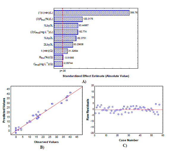
Figure 2A shows for the phenol degradation (PD), the Pareto Diagram with the effects that are statistically significant. The effects whose angles are the right of the divider (p>0.05) are considered significant, are these: “t(L), t(Q), RP/H(L), CPH0(Q), CPH0(L), RP/H(Q)” and the interactions “2L by 3L” and “1L by 2L”. However, the interaction “1L by 3L” this within an uncertainty with p<0.05.
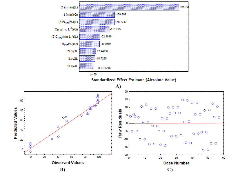
Figure 2B presents the adjustment between the predicted values (simulated) and observed values (experimental) by the model to get the best response as regards Phenol Degradation (PD) of almost 100%. This shows that the points are well distributed along the trendline, in an operating range that varies from about 0.00 to 99.61%. It was observed that the predicted result was almost the same as the experimental analysis and the error between the two was less than 5%. The coefficient of multiple determinations (R2), which represents the proportion of the variation of the studied parameters being described through the set of selected explanatory variables, showed values greater than 0.99. The adjusted R2 is the percentage of variation in the response that is explained by the model, adjusted for the number of model predictors in relation to the number of observations, presented values greater than 0.98 (98%) demonstrating the excellent response capacity of the model proposed directly impacting on the low residual error and its uniform distribution (Figure 2C and 2D).
Figure 2C indicates the residual distribution to analyze the dispersion of the data with the values of deviations (data calculated on the basis of experimental data) well distributed around the axis of abscissas for the response of phenol degradation. In this, it is possible to verify that the data did not show dispersions trends relative to the x axis (zero point), so this model satisfactorily represents the behavior of the process within the domain.
To analyze the mathematical model, adjustments to the points were made by nonlinear regression methods. The application of Response Surface Methodology (RSM) offers, on the basis of parameter estimation, the Equation (12) like empirical relationship between the Phenol Degradation rate, YPD, and independent variables studied.
= − + − + − + − −
0.0001 0.0001 0.0002 x x x x x x + +
1 2 1 3 2 3
(12)
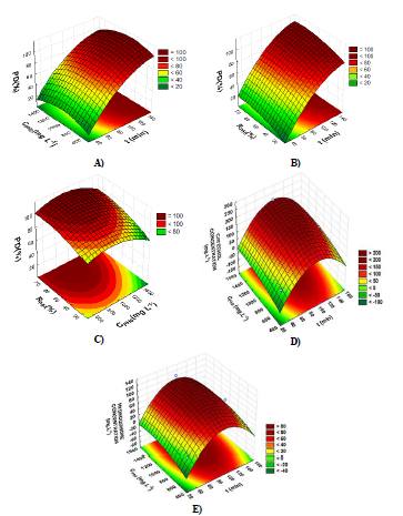
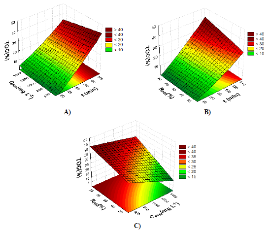
Figure 3: A) PD as a function of (CPh0) and (t); B) PD as a function of (RP/H) and (t); C) PD as a function of (RP/H) and (CPh0); D) Evolution of catechol concentration as a function of (CPh0) and (t); E) Evolution of hydroquinone concentration as a function of (CPh0) and (t). P=38.6 kW, E=10%, QL=170 L h-1 and t=30-150 min.
Figure 3A, B and C shows the response surface methodology from the simulated data of the by means of statistical analysis of phenol degradation. Figure 3A indicates only <20% of phenol degradation was attained in 30 min of process time, independently of CPH0 (500, 1000 and 1500 mg L-1). However, increasing the operation time to 150 min the total phenol degradation is almost completely achieved in 100%, for RP/H between 50% and 75%, independently of CPH0.
Figure 3B indicates the lowest values, <20% of the phenol degradation was attained in 30 min of process time, independently of RP/H (25, 50 e 75%), but the increase of the time to 150 min obtained the total phenol degradation, 100%, for RP/H between 50% and 75%, independently of CPH0 (500, 1000 and 1500 mg L-1). This can be explained due to the amount of hydrogen peroxide added [40].
Figure 3C presents a low phenol degradation, <80%, in 90 min of process time, for RP/H of 25%, independently of CPH0 (500, 1000 and 1500 mg L-1). However, in 150 min of process time, for RP/H >50%, independently of CPH0, obtained the total phenol degradation, 100%. Regardless of the value of the initial phenol concentration, CPh0, of 500, 1000 and 1500 mg L-1 and to the molar stoichiometric ratio of phenol/ hydrogen peroxide, RP/H, of 75%, the process presents maximum rates of phenol degradation almost 100% in t=150 min of operation.
The phenol oxidation occurred based on the change in the liquid phase coloration with reaction time (see Figure 1C). Resolution 430 of the Conselho Nacional do Meio Ambiente-CONAMA (National Council on the Environment), Brazil set a maximum total concentration of phenols of 0.5 mg.L-1 for all effluents originating from any polluting source that can be disposed of in water bodies as of 13 May 2011 [22].
Figure 3D and E shows the dynamic concentration evolution of the intermediates formed, catechol and hydroquinone, respectively, which are products of the thermochemical oxidation of phenol, according to the mechanism given by Devlin and Harris [54, 55]; however, catechol shows a more accentuated profile than the profile of hydroquinone. These products were formed after 30 min of phenol consumption until 100 min of reaction, being then reduced the concentration of these intermediaries and as the process progressed 1,4-dioxo-2-butene, alkenes, and glyoxal, aldehydes, were likely the products in the reaction mixture that were formed from of the hydroquinone and catechol/ hydroquinone degradation, respectively [55]. Similar results were reported by Lipczynska-Kochany [56] and Alnaizy and Akgerman [57]. There are parallel reactions that compete for the same reactants and therefore a higher concentration is expected for the reaction that generates more products, such as carboxylic acids, alkenes and aldehydes.
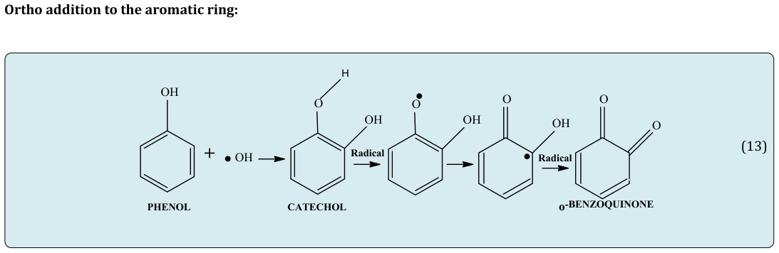
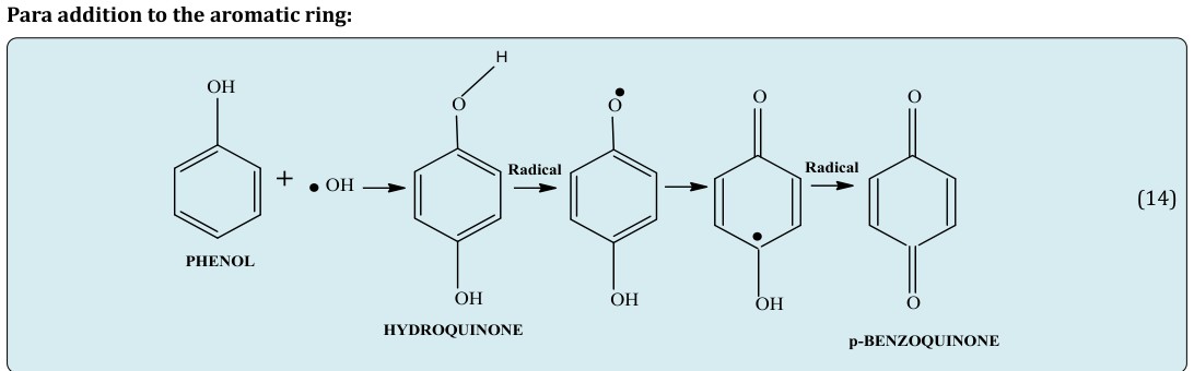
The phenol degradation and formation of intermediates following the break in the aromatic ring way result from an excess of hydroxyl radicals [58]. Thus, in the first oxidation step, the increased catechol production followed by the formation of o-benzoquinone may have been instigated by mesomeric properties (electronic effects resulting by the phenomenon of resonance in a series of components), leading to the re-distribution of electrons to the ortho position, which can increase the reactivity of this part of the structure due to the nearness of differing charges [59], following to the Equation (13). The next phase, para addition, includes the increased hydroquinone production followed by the formation p-benzoquinone and depends on the position at which the hydroxyl radical attacks the aromatic ring (mesomeric effect) [60], according to the Equation (14):
Brandão, et al. [26] studied the effect of burner power dissipated (19.3, 29.0 and 38.6 kW) and air excess (10 and 40%). The optimal conditions for phenol degradation were then identified: burner power dissipated 38.6 kW and air excess of 40%, thus reaching phenol degradation values of 100%. The complete phenol degradation can be achieved after 225 min of process operation, regardless of the air excess value (10 or 40%) and burner power dissipation (29 or 38.6 kW). The increase in the burner power dissipated from 19.3 to 38.6 kW allows the reduction of the operational time of the process for a phenol degradation of 100%. The concentrations of hydroquinone and catechol formation obtained using the burner power dissipated of 38.6 kW are lower compared to those quantified with the power of 29 kW, for the same excess of air of 10%.
Amado-Piña [61] investigated the phenol degradation in three conditions: ozonation (O3), Electro-Oxidation (EO) and ozonation-electro-oxidation (O3-EO) combined method. The more high phenol mineralization with values above than 99.8%, practically, was obtained with use of the combined effects (O3-EO) under pH 7.0 ± 0.5, at a current density of 60 mA cm−2, 0.05 L min−1 flow rate, ozone concentration of 5 ± 0.5 mg.L−1. This process lets to detect the highest degrees of mineralization and eliminates the toxicity of the samples.
Barik and Gogate [62] reviewed the application of hybrid treatment including AOP/Hydrodynamic Cavitation- HC for degradation of 2,4,6-trichlorophenol (2,4,6-TCP). The degradation efficiency was obtained with use of the combined effects: HC/H2O2, HC/O3, O3/H2O2 and HC/O3/ H2O2, reaching values above than 95% degradation with use of HC/O3 and O3/H2O2 processes. The complete degradation by Chemical Oxygen Demand (COD) practically was achieved and a TOC decrease was obtained representing 80.95% with use of HC/O3/H2O2 process, being an efficient method for hybrid treatment containing 2,4,6-trichlorophenol.
Renuka and Gayathri [63] examined a polymer supported containing: Fe(PS-BBP)Cl3 [PS = chloromethylated polystyrene divinyl benzene; BBP = 2,6-bis (benzimidazolyl) pyridine] to evaluate the degradation of phenolic compounds and dyes, in 30 and 120 min respectively, under the efficiency of AOPs including ultravioleta/hydrogen peroxide (UV/H2O2). The photodegradation efficiency was practically 100%. The mineralization rates were obtained by Chemical Oxygen Demand (COD) trials representing the efficiency of the process, indicating 96 and 100% mineralization conversion of phenol and methyl orange, respectively.
Figure 4A shows for the TOC conversion, the Pareto Diagram with the effects that are statistically significant. The effects whose angles are the right of the divider (p>0.05) are considered significant, are these: “t(L), t(Q), RP/H(L), RP/H(Q), CPH0(L)” and the interactions “1L by 2L”, “1L by 3L” and “2L by 3L”. However, the effects “CPH0(Q)” this within an uncertainty with p<0.05.
Figure 4B presents the adjustment between the predicted values (simulated) and the observed values (experimental) by the model to get the best response as regards TOC exceeding 40%. This shows that the points are well distributed along the trendline, in an operating range that varies from about 0.00 to 40.57%. It was observed that the predicted result was almost the same as the experimental analysis and the error between the two was less than 5%. For the coefficient of multiple determinations (R2) and the adjusted R2 that had their values greater than 0.96 as well as uniform distribution in the residual error, the model can be considered satisfactory in its predictions.
Figure 4C indicates the residual distribution to analyze the dispersion of the data with the values of deviations (data calculated on the basis of experimental data) well distributed around the axis of abscissas for the response of TOC. In this, it is possible to verify that the data did not show dispersions trends relative to the x axis (zero point), so this model satisfactorily represents the behavior of the process within the domain.
To analyze the mathematical model, adjustments to the points were made by nonlinear regression methods. The application of Response Surface Methodology (RSM) offers, on the basis of parameter estimation, the Equation (15) like empirical relationship between the TOC rate, YTOC, and independent variables studied.
2 2 2 1 1 2 2 3 3 1 2
5.782 0.123. 0.001 0.006 0.000 0.262 0.000 0.000
TOC Y x x x x x x x x = + + − − − − −
0.003 0.000 x x x x + +
1 3 2 3 (15) Figure 5A, B and C shows the response surface methodology from the simulated data of the by means of statistical analysis of TOC conversion. Figure 5A shows that the speed of the rate of reduction of organic load increases with increased, t, and that from 150 min, the TOC conversion was practically more than 40%, regardless of CPh0; In addition, with a (t) less than 120 min, the TOC conversion begins to decrease and is around <30% independent of CPh0.
Figure 5B shows that the speed of the rate of reduction of organic load increases with increased, t, and that from 150 min, the TOC conversion was practically more than 40%, for RP/H of 75%; thus, this test corresponded to the best operational condition for DiCTT thermochemical oxidation [40]. In addition, with a RP/H less than 50%, the TOC conversion begins to decrease and is around <30% for (t) less than 120 min.
Figure 5C shows that the highest percentage mineralization (>40%) was obtained using a large quantity of free hydroxyl radicals (•OH) in the media, a RP/H of 75%, which provided the best process conditions. In addition, with a RP/H less than 50%, the TOC conversion begins to decrease and is around 35% for values of CPh0, less than 1200 mg L-1. Just as, for the higher concentrations of phenol, above 1200 mg L-1, and RP/H decreasing of 50 for 25%, the TOC conversion is less than 15%. Using an equivalent concentration of hydrogen peroxide at the molar stoichiometric ratio of phenol/peroxide was essential for preventing the destructive effects that can be caused by an excess of this oxidizing agent during the reaction with phenol [64]. Data reported in the literature demonstrated in organic compounds that during treatment by AOPs (UV/H2O2) high degradation efficiency was observed in the percentage removal of the compound with less time of treatment [65].
Brandão, et al. [47] analyzed the effect of initial phenol concentration, CPh0, of 500, 2000 and 3000 mg.L−1. The experiments studies were performed using a molar stoichiometric ratio of phenol/hydrogen peroxide, RP/H, of 50%, an air excess, E, of 40%, a combustion gas recycling rate, QRG, of 50%, a liquid phase flow rate (QL) of 170 L.h−1, and, a natural gas flow, QGN, of 4 m3 h−1, on the oxidation of phenolic effluents by DiCTT. The complete degradation of phenol, almost 100%, was obtained independently of CPh0 over a 170-min period. A TOC conversion of almost 35% was obtained to time of 210 min. A time of 110 min was identified from the concentration profiles of hydroquinone and catechol. The concentrations of these intermediates decreases independently of CPh0, indicating the formation of the other organic substance, which were not acids, constant pH, such as, 1,4-Dioxo-2-buteno and Glyoxal.
Berenguer, et al. [66] studied the effect of Temperature (T), Stoichiometric Molar Ratio Phenol/Hydrogen Peroxide (R), Air Flow (QAR) and pH of a liquid effluent containing the synthetic organic compound (phenol) with an initial concentration (CF0) of 500 mg.L-1, in a laboratory-scale batch reactor, model type PARR. A degradation of the phenol above 99% and a conversion of the TOC greater than 70% were respectively obtained under the optimum operating conditions of the process (T=90°C, R=100%, pH=7 and QAR=100 NL.h-1).
Chandana and Subrahmanyam [67] investigated the liquid phase phenol degradation and mineralization by using an atmospheric pressure plasma reactor operating under argon (Ar)/air plasma. The addition of CeO2, Ce0.90Ni0.10O2-δ and 10 wt% NiO/CeO2 catalysts better the efficiency of phenol degradation. The results indicated that Ar plasma allows the degradation due to the formation of hydroxyl radicals (•OH) in the presence of a solid catalyst, being the better results for the degradation and mineralization of phenol with 71 mg.L−1 of H2O2, 1.5 × 10⁻⁶ Molar s-1 of •OH production rate. The use of catalyst Ce0.90Ni0.10O2-δ + Fe2+ obtained the phenol degradation and mineralization efficiency up to 99% and 61% for 300 mg.L−1 of phenol and it was observed a combination to plasma that showed the highest efficiency of 24 g kWh-1 due to the formation of of •OH, indicating the formation of the stable intermediates, benzoquinone and hydroquinone.
Modeling the Data Set Generated by the ANN for Phenol Degradation and TOC Conversion
Artificial neural network (ANN) application is typically used for optimization and process modeling [68]. ANNs have been applied in a total of 20 experimental data points, containing five replications at the central point to determine optimized process conditions using microwave technique for the extraction of natural dye from dried pomegranate rind. Following trial, it was analyzed that 10 neurons produce minimum result of error of the training and validation sets. The network showed a perfect model with correlation coefficient (R) approximately 1 between the prediction of the model and the experimental results trained from the input data using error backpropagation algorithm [69]. ANN modeling was used and the number of experimental trials was 27 for removal of high concentration of sulfate from pigment industry effluent by chemical precipitation using barium chloride. ANN prediction by the model was evaluated and it exhibited good performance (R2 value 0.9986). The network architecture consisted of one input layer with 3 inputs, one hidden layer with 10 neurons and an output layer [70].
In this study, ANN building were chosen as a Multi- Layer Perceptron (MLP) feed-forward networks that were trained by input-output data using the backpropagation algorithm [68]. For the ANN used through mathematical modeling with the configuration of an MLP network, the number of neurons tested in the Hidden Layer was varied between 3-11. The number of neurons in the hidden layer is established from the precision intended for neural predictions, possibly being used as a measure in the neural network model. In the next step, ANN model was applied to predicate the optimized parameters required for maximizing the removal efficiency of phenol and a TOC mineralization [8].
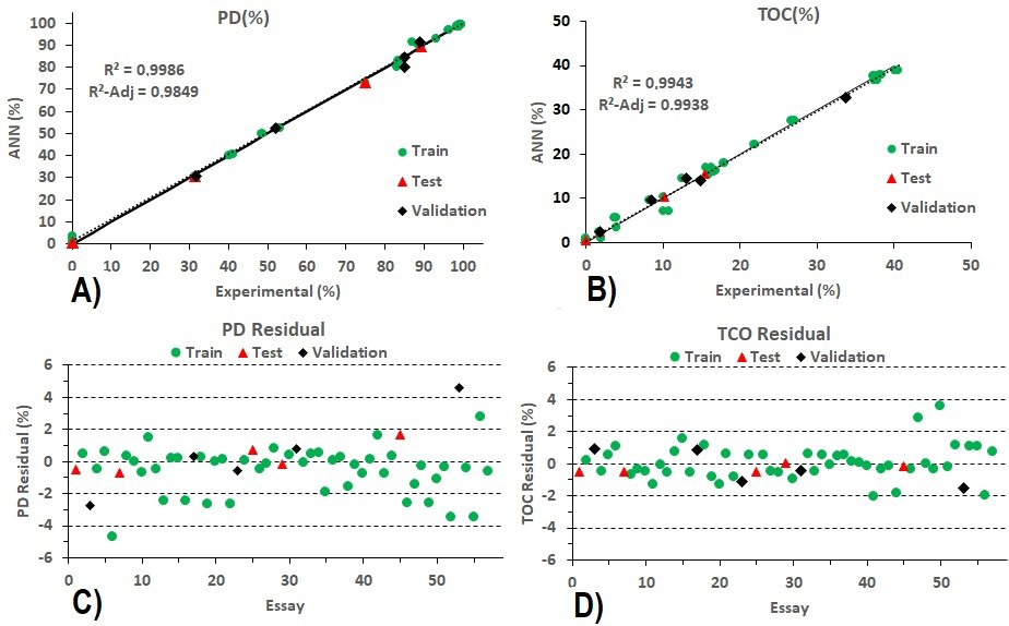
When an incomplete number of samples are accessible, proceeding to develop nonlinear pattern identification methods (such as ANN’s) which can model the complex biological, environmental and instrument variation can be considered as a better solution to develop robust models [71]. The type of ANN that uses a back-propagation perceptron with controlled learning is defined by layered architectures, and feed-forward connections between neurons or back-connections [72]. The neural network is a tool that is useful in problem solving, being deployed from a set of biological model with computational technique that contains of some processing units in the system. ANN has a arrangement constituted of small computational units called artificial neurons [73]. In this research, the selection of the best model for ANN was established from the average of the smallest quadratic errors in training, testing and validation that was developed to predict the relationship between the experimental variables: the degradation efficiency and TOC conversion. Total 57 experimental data points was taken for to generate the ANN and nearly 5,000 neural networks were trained, out of which the best 6 results were chosen for the assessment [69]. The training was used to adjust the ANN weights and the test to evaluate the neural network configuration, in which 80% of the data were used for the formation of the network in the training, 10% for testing and 10% for validation. The Root Mean Squared (RMS) was calculated with 6 neurons in the hidden layer and were obtained the following results, considering the lowest average quadratic error form 6 best models: for PD residual (1.61% for all data, 1.56% for Train, 0.89% for Test and 2.44% for Validation) and for TCO residual (1.02% for all data, 1.07% for Train, 0.38% for Test and 1.01% for Validation). Thus, the network had a 3:6:2 configuration.
In this research, for the ANN with MLP model was used the hyperbolic tangent activation function for the network input and the sigmoidal logistic activation function for the network output, being this technique quite efficient to get the optimal conditions for this DiCTT method. In the MLP network configuration, the principle of the error backpropagation algorithm is to calculate the error in the network output, then back to the intermediate layers in order to perform the adjustment of the weights proportional to the values of the connections between the layers. The sigmoidal (nonlinear) functions of each neuron both in the intermediate layers and in the composition of its structure in successive layers of the network, are usually used for an approximation of the degree function due to the possibility of the descending gradient requiring the use of continuous and differential activation functions, characteristic of an “MLP”.
Table 3 shows the values of the weights (wij) of the input variables, output and the hidden layer obtained by Artificial Neural Network (ANN) for the experimental complete factorial design type with factorial k, 23. This ANN was obtained a Multilayer Perceptron, MLP-type, like the logistic-type (also called log-sigmoidal or logsig), with a 3:6:2 structure representing three data in the input (initial phenol concentration, molar stoichiometric ratio Phenol/ Hydrogen peroxide and the reaction time), six neurons in the hidden layer and two data (results) in the output (Phenol Degradation and TOC conversion). These results were achieved using statistic software version 8.0.
The ANNs present good results, with slopes of approximately 1, near-zero Intercepts, R2 values near 0.99 and a standard error close to 1. Several iterations were conducted with different numbers of neurons in the hidden layer to determine the best ANN structure.
| Connections | W 1 | W 2 | ||||
|---|---|---|---|---|---|---|
| N0 of neurons | C (mg.L-1) Ph0 | R (%) P/H | t (min) | Layer/ Input (Bias) | PD | TOC |
| 1 | 1.0376 | 0.2827 | 4.1141 | -1.185 | 1.1208 | 0.1322 |
| 2 | 1.5555 | -1.467 | -2.9247 | 1.2657 | -2.3658 | -7.9059 |
| 3 | -1.7787 | -2.1614 | -1.2651 | 3.7011 | -3.6215 | -1.2745 |
| 4 | -5.1935 | -0.008 | -4.9088 | 2.0681 | -4.5156 | -2.6658 |
| 5 | -2.1805 | 0.6661 | 1.2917 | -0.7701 | -4.9369 | -6.3325 |
| 6 | 0.551 | -5.4344 | -3.9446 | 0.3775 | -4.75 | -5.6763 |
| - | - | - | - | Hidden Layer/(Bias) | 12.3936 | 6.9208 |
Table 3: Values of the weights between the input and the hidden layers, W1, and output layer, W2, for the Phenol Degradation of (
In order to observe once again the consistency of the results obtained by ANN, the graphs were generated from the calculated data presented according to the experimental results, for the training, test and validation data set. With the produced graphs, the linear correlation factor (R2) for the configuration of the analysed networks was obtained through a linear adjustment.
Figure 6A and B show the data calculated according to the experimental results for the data set (training, testing and validation) used in ANN to obtain Phenol Degradation (PD) and TOC conversion, respectively. In these were verified a good alignment of the data obtained in the ANN to the linear adjustment line, indicating that also for a number of iterations (Ni) of 1000 used in the calibration of the neural network and a number of Neurons in the Hidden Layer (NHL) of 6, the alignment of the data represents well the behaviour of the system.
The ANN with an index of 6 contains few neurons in the hidden layer and was selected as the best ANN, with good results for R2 (0.9983 for Training, 0.9999 for Testing and 0.9958 for Validation). The algorithms used to optimise the network were the almost Newton method of the type BFGS (Quasi-Newton method with the Hessian approximation proposed by Broyden, Fletcher, Powell and Goldfarb).
Figure 6A and 6B show that R2-adjusted is observed very close to R2. This indicates that the curve is not biased. The results obtained in the construction of the neural network were accurate and satisfactory, as evidenced by the R2 value and the validation test. The R2-adjusted coefficient is represented by Equation 16, being exemplified by a changed correlation coefficient R2 that checking account for the number of independent variables and data set extent.
( ) ( ) 2 2 1 1 1 1 Adj n R R n k − = − ⋅ − − + (16)
where n denotes the data set extent, and k denotes the number of independent variables.
Figure 6C and 6D show from a clearer analysis that the dispersion of the data was generated with the values of the deviations (data calculated according to the experimental data) by the ANN and that it’s are well distributed around the axis of the abscissas for the 6 neurons in the hidden layer.
Figure 6C demonstrates a small more dispersion in the training, testing and validation of ANN (for phenol degradation) in relation to the x-axis when compared to Figure 6D (for TOC Conversion). Although, these results are still quite satisfactory for this ANN, considering that the linear correlations are greater than 99% and most of the data are still near to the zero point.
Figure 6D confirms that the data do not indicate dispersion trends in relation to the x-axis (zero point) in ANN (for TOC conversion). Thus, the ANNs model presents satisfactorily once again the behaviour of the process being well distributed in the domain of experimental data.
Brandão, et al. [40] studied the thermochemical oxidation phenol and it’s was monitored from oxidative degradation to the mineralization of the organic compound and the formation of acids. The concentrations of phenol, catechol, hydroquinone and para-benzoquinone were monitored by High performance Liquid Chromatography (HPLC), a Total Organic Carbon (TOC) analyzer and the hydrogen potential (pH) using a pH meter. The following operational parameters were performed: The liquid phase flow rate (QL) of 170 L.h-1, a burner power dissipation (P) of 38.6 kW at an 10% air excess (E) of 10 %, an initial phenol concentration (CPh0) of 500 mg.L−1 and a recycle rate of gaseous thermal wastes (QRG) of 50%. The organic pollutant (phenol) was degraded (almost 100%) over a 150-min period and a TOC mineralization of approximately 60% was observed corresponding to an operational time of 210 min at a RP/H of 75%, which was considered to be the best operating condition for the DiCTT process. The ANN computational tool was later used with a “Neural Networks” module to predict the phenol degradation, the TOC conversion and the temporal velocity profile of phenol degradation, as a function of time, respectively. The best MLP-type ANN model used 7 neurons in the hidden layer to predict the most accurate response. Thus, the network showed a 2:7:3 configuration for a correlation coefficient (R2) of 0.999 for phenol degradation and the TOC conversion and R2 of 0.997 for temporal velocity profile of phenol degradation.
Conclusion
The present work used an empirical matematical modeling for phenol degradation and TOC conversion by the thermochemical oxidation of the effluents using Direct Contact Thermal Treatment process. The developed model establishes some chemical reactions and formations of organic compounds, being able to predict phenol oxidation in the ortho and para positions, resulting in aromatic isomers that are catechol and hydroquinone, as well as other chemical species, such as: carboxylic acids, alkenes and aldehydes. Sensitivity analysis was performed on the matematical parameters to determine those that are most influential in the phenol oxidation, catechol and hydroquinone concentrations. As expected, the most influential parameters are that regulate the oxidation by hydroxyl radical reactions involving these studied compounds.
The parameter estimation was performed to best fit the experimental data and the overall correlation coefficient obtained from the model developed by Response Surface Methodology (RSM) that was 0.9444-0.9725 for both, phenol degradation and TOC conversion, respectively. It was shown that of the three RP/H used in the experiments, RP/H of 75%, independent of the CPh0, was able to meet the best CONAMA standard for maximum concentration of residual aromatic compounds, showing practically 100% of phenol degradation and more 40% of TOC conversion after 150 min. The graphs of the comparison between calculated and experimental values of the output variable and the deviations obtained for the data set related to learning, testing and validation by ANN model simulation showed that the optimum condition for complete phenol degradation and more 40% of TOC conversion was obtained at RP/H of 75%. The results data corroborates the experimental data in this research. The Root Mean Squared (RMS) was calculated with 6 neurons in the hidden layer and was obtained the following results: for PD residual (1.61% for all data, 1.56% for Train, 0.89% for Test and 2.44% for Validation) and for TCO residual (1.02% for all data, 1.07% for Train, 0.38% for Test and 1.01% for Validation). The best MLP-type ANN model used 6 neurons in the hidden layer to predict the most accurate response for phenol degradation and TOC conversion, respectively. Thus, the network showed a 3:6:2 configuration for a correlation coefficient (R2) of 0.99 for phenol degradation and the TOC conversion, respectively.
In these conditions, the reaction medium temperature reached approximately 78 0C, thus, it became the controlling factor in the TOC conversion, as well as other operational parameters, including the molar ratio of phenol/peroxide. The present developments include the integrated optimisation of the process consisting of a termochemical oxidation, as well as the extension of the model to DiCTT process. This new technology is attractive because natural gas is used as the energy source, and phenolic compounds can be oxidized at low temperatures, atmospheric pressure and the reagent used for the generation of hydroxyl radicals, hydrogen peroxide, is cheap, to initiate the phenol oxidation in the aqueous phase, the natural gas is available in off-shore petroleum platforms and configuration reactor requires limited space. All these advantages make the DiCTT process, potentially efficient method, allows integrating the advanced oxidation processes existing in the industrial practice.
Acknowledgments
The authors wish to thank the Financiadora de Estudos e Projetos – FINEP/Ministry of Science and Technology- MCT-Brazil and PETROBRÁS for providing financial support during the development of this research and the Conselho Nacional de Desenvolvimento Científico e Tecnológico - CNPq for awarding the research grants.
References
-
Chu, L, Yu S, Wang J (2016) Gamma radiolytic degradation of naphthalene in aqueous solution. Radiat Phys Chem 123: 97-102.
-
Ganguli A, Ganguly P, Das P, Saha A (2020) Integral approach for the treatment of phenolic wastewater using gamma irradiation and graphene oxide. Groundw Sustain Dev 10: 100355.
-
Oller I, Malato S, Sánchez-Pérez JA (2011) Combination of Advanced Oxidation Processes and biological treatments for wastewater decontamination—A review Sci Total Environ 409: 4141-4166.
-
Carvalho MN, Motta M, Benachour M, Sales DCS, Abreu CAM (2012) Evaluation of BTEX and Phenol Removal from Aqueous Solution by Multi-Solute Adsorption Onto Smectite Organoclay. J Hazard Mater 239-240: 95- 101.
-
Panico A, Basco A, Lanzano G, Pirozzi F, Santucci de Magistris F, et al. (2017) Evaluating the structural priorities for the seismic vulnerability of civilian and industrial wastewater treatment plants. Saf Sci 97: 51- 57.
-
Mukherjee M, Goswami S, Banerjee P, Sengupta S, Das P, et al. (2019) Ultrasonic assisted graphene oxide nanosheet for the removal of phenol containing solution. Environ Technol Innovation 13: 398-407.
-
Park Y, Skelland AHP, Forney LJ, Kim JH (2006) Removal of phenol and substituted phenols by newly developed emulsion liquid membrane process. Water Res 40(9): 1763-1772.
-
Razzaghi M, Karimi A, Ansari Z, Aghdasinia H (2018) Phenol Removal by HRP/GOx/ZSM-5 from aqueous solution: Artificial neural network simulation and genetic Algorithms optimization. J Taiwan Inst Chem Eng 89: 1-14.
-
Praveen P, Loh KC (2016) Osmotic membrane bioreactor for phenol biodegradation under continuous operation. J Hazard Mater 305: 115-122.
-
Araújo MC (2003) Cinética experimental e resistências difusionais na oxidação úmida de compostos fenólicos utilizando catalisadores metálicos. Dissertação de Mestrado, UFRN, Natal, Brazil, pp: 100.
-
Chen IP, Lin SS, Wang CH, Chang JS, Chang EL (2004) Preparing and characterizing an optimal supported ceria catalyst for the catalytic wet air oxidation of phenol. Appl Catal B 50(1): 49-58.
-
Tor A, Cengeloglu Y, Aydin ME, Ersoz M (2006) Removal of phenol from aqueous phase by using neutralized red mud. J Colloid Interface Sci 300(2): 498-503.
-
Zhou GM, Fang HP (1997) Co-degradation of phenol and m-cresol in a UASB reactor. Bioresour Technol 61(1): 47-52.
-
Guerra R (2001) Ecotoxicological and chemical evaluation of phenolic compounds in industrial effluents. Chemosphere 44(8): 1737-1747.
-
Mishra VS, Mahajani VV, Joshi JB (1995) Wet air oxidation. Ind Eng Chem Res 34(1): 2-48.
-
Agency for Toxic Substances and Disease Registry (ATSDR) (2006) Toxicological profile for phenol. U.S. Department of Health and Human Services, Atlanta, GA, USA.
-
Shanmuganathan S (2016) Artificial neural networks modelling: An introduction. In: Shanmuganathan S, et al. (Eds.), Artificial neural networks modelling. 1st(Edn.), Springer, Cham, pp: 14.
-
Reible D (2017) Fundamentals of environmental engineering. 1st(Edn.), CRC Press, Boca Raton, pp: 544.
-
Monier E, Paltsev S, Sokolov A, Chen YHH, Gao X, et al. (2018) Toward a consistent modeling framework to assess multi-sectorial climate impacts. Nat Commun 9(1): 1-8.
-
Britto JM, Rangel MC (2008) Processos avançados de oxidação de compostos fenólicos em efluentes industriais. Quim Nova 31(1).
-
Suthersan SS, Horst J, Schnobrich M, Welty N, McDonough J (2016) Remediation engineering: Design concepts, CRC Press, pp: 627.
-
CONAMA (2011) Ministério do Meio Ambiente. Conselho Nacional de Meio Ambiente (CONAMA), Brasília, DF, Resolução n0 430.
-
Pintar A, Levec J (1992) Catalytic liquid-phase oxidation of refractory organics in waste water. Chem Eng Sci 47 (9-11): 2395-2400.
-
Kolaczkowski ST, Beltran FJ, Mclurgh, DB, Rivas FJ (1997) Wet Air Oxidation of Phenol: Factors that May Influence Global Kinetics. Process Saf Environ Prot 75(4): 257-265.
-
Brandao YB (2012) Thermal Treatment by Direct Contact (dictt) of Phenolic Liquid Effluents in a Semi- industrial Plant: Experimental Study and Modeling of the Process by Artificial Neural Networks. Doctorate Thesis, Federal University of Pernambuco, Recife- Brazil, pp: 276.
-
Brandao Y, Teodosio J, Benachour M, Oliveira J, Marinho I, et al. (2010) Study of the effect of excess air and the dissipated power of the burner on the capacities of the DiCTT process in the treatment of phenolic liquid effluents. Sist Cib Inf 7(2): 1-9.
-
Kim KH, Ihm SK (2011) Heterogeneous catalytic wet air oxidation of refractory organic pollutants in industrial wastewaters: A review. J Hazard Mater 186(1): 16-34.
-
Mert BK, Yonar T, Kilic MY, Kestioglu K (2010) Pre- treatment studies on olive oil mill effluent using physicochemical, Fenton and Fenton-like oxidations processes. J Hazard Mater 174(1-3): 122-128.
-
Bilinska L, Gmurek M, Ledakowicz S (2017) Textile wastewater treatment by AOPs for brine reuse. Process Saf Environ Prot 109: 420-428.
-
Alkaram UF, Mukhlis AA, Dujaili AHA (2009) The removal of phenol from aqueous solutions by adsorption using surfactant-modified bentonite and kaolinite. J Hazard Mater 169(1-3): 324-332.
-
Castro IU, Stuber F, Fabregat A, Font J, Fortuny A, et al. (2009) Supported Cu(II) polymer catalysts for aqueous phenol oxidation. J Hazard Mater 163(2-3): 809-815.
-
Gorska P, Zaleska A, Hupka J (2009) Photodegradation of phenol by UV/TiO2 and Vis/N,C-TiO2 processes: Comparative mechanistic and kinetic studies. Sep Purif Technol 68(1): 90-96.
-
Liu H, Liang MY, Liu CS, Gao YX, Zhou JM (2009) Catalytic degradation of phenol in sonolysis by coal ash and H2O2/O3. Chem Eng J 153(1-3): 131-137.
-
Luis AMD, Lombrana JI, Menendez A, Sanz J (2011) Analysis of the Toxicity of Phenol Solutions Treated with H2O2/UV and H2O2/Fe Oxidative Systems. Ind Eng Chem Res 50(4): 1928-1937.
-
Yang B, Ying GG, Zhao JL, Zhang LJ, Fang YX (2011) Oxidation of triclosan by ferrate: Reaction kinetics, products identification and toxicity evaluation. J Hazard Mater 186(1): 227-235.
-
Grcic I, Papic S, Koprivanac N, Kovacic I (2012) Kinetic modeling and synergy quantification in sono and photooxidative treatment of simulated dyehouse effluent. Water Res 46(17): 5683-5695.
-
Vallejo M, San Roman MF, Ortiz I, Irabien A (2015) Overview of the PCDD/Fs degradation potential and formation risk in the application of advanced oxidation processes (AOPs) to wastewater treatment. Chemosphere 118: 44-56.
-
Zhang T, Cheng L, Ma L, Meng F, Arnold RG, et al. (2016) Modeling the oxidation of phenolic compounds by hydrogen peroxide photolysis. Chemosphere 161: 349- 357.
-
Li X, Zhou M, Pan Y, Xu L, Tang Z (2017) Highly efficient advanced oxidation processes (AOPs) based on pre- magnetization Fe0 for wastewater treatment. Sep Purif Technol 178: 49-55.
-
Brandao Y, Teodosio J, Dias F, Eustaquio W, Benachour M (2013) Treatment of phenolic effluents by a thermochemical oxidation process (DiCTT) and modelling by artificial neural networks. Fuel 110: 185- 195.
-
Benali M, Hugron I, Morin M, Guy C (2000) Novel gas technology for treatment of hazardous aqueous waste streams. Proceedings of Symposium on Energy Engineering in the 21st Century (SEE2000) Volume I-IV, Begell House Inc publishers, Danbury, Connecticut, United States, pp: 1412-1419.
-
Benali M, Guy C (2007) Thermochemical oxidation of phenolic-laden liquid effluent models. J Environ Eng Sci 6(5): 543-552.
-
Barros Neto B, Scarminio IS, Bruns RE (2010) Como fazer experimentos. 4th(Edn.), Bookman, Porto Alegre, Brazil, pp: 413.
-
Sinha K, Das PS, Datta S (2012) Response surface optimization and artificial neural network modeling of microwave assisted natural dye extraction from pomegranate rind. Ind Crop Prod 37(1): 408-414.
-
Yang Y, Zhou Z, Lu C, Chen Y, Ge H, et al. (2017) Treatment of chemical cleaning wastewater and cost optimization by response surface methodology coupled nonlinear programming. J Environ Manage 198(Part 2): 12-20.
-
Poznyak A, Chairez I, Poznyak T (2019) A survey on artificial neural networks application for identification and control in environmental engineering: Biological and chemical systems with uncertain models. Annual Reviews in Control 48: 250-272.
-
Brandão YB, Oliveira JGC, Benachour M (2017) Phenolic Waste waters: Definition, Sources and Treatment Processes. In: Marcos SH, et al. (2017) Phenolic Compounds: Natural Sources, Importance and Applications. Intech, Rijeka-Croatia, pp: 323-342.
-
Kasiri MB, Aleboyeh H, Aleboyeh A (2008) Modeling and optimization of heterogeneous photo-fenton process with response surface methodology and artificial neural networks. Environ Sci Technol 42(21): 7970-7975.
-
Oliveira, Correia de JG (2009) Estudo teórico- computacional por via CFD e experimental da combustão do gás natural para tratamento de efluentes orgânicos líquidos aplicando a nova tecnologia DICTT. Masters Dissertation, University Federal of Pernambuco, Recife- Brazil, pp: 153.
-
Copergás (2009) Companhia Pernambucana de Gás.
-
Chaves ATCA (2008) Otimização do processo de biodiesel etílico do óleo de girassol (Hellianthus annus) aplicando um delineamento composto central rotacional (DCCR). Masters Dissertation, University Federal of João Pessoa, Paraíba, Brazil.
-
Myers RH, Montgomery DC, Anderson-Cook CM (2002) Response Surface Methodology: Process and Product Optimization Using Designed Experiments. 4th(Edn.), John Wiley and Sons, New York, pp: 856.
-
Soleymani AR, Saiena J, Bayatb H (2011) Artificial neural networks developed for prediction of dye decolorization efficiency with UV/K2S2O8 process. Chem Eng J 170(1): 29-35.
-
Rodrigues MI, Lemma AF (2009) Design of experiments and process optimization. Casa do Espírito Amigo Fraternidade Fé e Amor, 2nd(Edn.), Campinas-São Paulo, Brazil.
-
Devlin HR, Harris IJ (1984) Mechanism of the oxidation of aqueous phenol with dissolved oxygen. Ind Eng Chem Res 23(4): 387-392.
-
Lipczynska-Kochany E (1993) Hydrogen peroxide mediated photodegradation of phenol as studied by a flash photolysis/HPLC technique. Environ Pollut 80(2): 147-152.
-
Alnaizy R, Akgerman A (2000) Advanced oxidation of phenolic compounds. Adv Environ Res 4(3): 233-244.
-
Alnaizy RS (1999) Mechanism and kinetic study for the hydroxyl free radicals mediated photoxidation of organic-contaminated-aqueous solutions. Pro Quest Dissertations Publishing, University of Texas, USA, pp: 9957386.
-
Teodosio JR (2010) Estudo e Otimização das Condições Operacionais do Processo de Oxidação Termoquímica DiCTT no Tratamento de Efluentes Fenólicos numa Planta Semi-Industrial. Federal University of Pernambuco, Recife, Brazil, pp: 96.
-
Amado-Piña D, Roa-Morales G, Barrera-Díaz C, Balderas- Hernandez P, Romero R, et al. (2017) Synergic effect of ozonation and electrochemical methods on oxidation and toxicity reduction: Phenol degradation. Fuel 198: 82-90.
-
Barik AJ, Gogate PR (2018) Hybrid treatment strategies for 2,4,6-trichlorophenol degradation based on combination of hydrodynamic cavitation and AOPs. Ultrason Sonochem 40(Part A): 383-394.
-
Renuka MK, Gayathri V (2018) UV/solar light induced photocatalytic degradation of phenols and dyes by Fe(PS-BBP)Cl3. J Photochem Photobiol A: Chem 353: 477-487.
-
Titus MP, Molina VG, Baños MA, Giménez J, Esplugas S (2004) Degradation of chlorophenols by means of advanced oxidation processes: a general review. Appl Catal B: Environ 47(4): 219-256.
-
Silva CRD, Maniero MG, Rath S, Guimarães JR (2016) Antibacterial Activity Inhibition after the Degradation of Flumequine by UV/H2O2. J Adv Oxid Technol 14: 106-114.
-
Berenguer CF, Brandão YB, Benachour M (2018) Estudo de Tratamento de água em Efluentes Refratários por Processo Fenton para Degradação e Mineralização desses Compostos em Reator de escala Laboratorial Modelo PARR. Anais da II MEMU, pp: 139-155.
-
Chandana L, Subrahmanyam Ch (2018) Degradation and mineralization of aqueous phenol by an atmospheric pressure catalytic plasma reactor. J Environ Chem Eng 6(3): 3780-3786.
-
Pandharipande SL, Aarti RD (2013) Artificial neural network approach for modeling f Ni (II) adsorption from aqueous solution using aegel marmelos fruit shell and syzygium cumini seed. IJAET 6(1): 114-127.
-
Kartic DN, Narayana BCA, Arivazhagan M (2018) Removal of high concentration of sulfate from pigment industry effluent by chemical precipitation using barium chloride: RSM and ANN modeling approach. J Environ Manage 206: 69-76.
-
Vidal MJM, Vázquez M (2015) Application of artificial neural networks coupled to UV–VIS–NIR spectroscopy for the rapid quantification of wine compounds in aqueous mixtures. CYTA – J Food 13(1): 32-39.
-
Allouche Y, López EF, Maza GB, Márquez AJ (2015) Near infrared spectroscopy and artificial neural network to characterise olive fruit and oil online for process optimisation. J Near Infrared Spectrosc 23(2): 111-121.
-
Silalahi DD, Reaño CE, Lansigan FP, Panopio RG, Bantayan NC (2016) Using genetic algorithm neural network on near infrared spectral data for ripeness grading of oil palm (Elaeis guineensis jacq.) fresh fruit. Inf Process Agric 3(4): 252-261.
-
Kuang B, Tekin Y, Mouazen AM (2015) Comparison between artificial neural network and partial least squares for on-line visible and near infrared spectroscopy measurement of soil organic carbon, pH and clay content. Soil Tillage Res 146(Part B): 243-252.
-
Gabriëls SHEJ, Mishra P, Mensink MGJ, Spoelstra P, Woltering EJ (2020) Non-destructive measurement of internal browning in mangoes using visible and near-infrared spectroscopy supported by artificial neural network analysis. Postharvest Biol Technol 166: 111206.
- Nigeria’s Vulnerability in the Face of Global Energy Policy
- A Simulation Study of Investigation of Optimum Oil Production Performance by Applying Various Gas Injection Methods in Oil Reservoir
- Characterization of Permo-Triassic Reservoirs through Thermal Maturity Assessment of Westphalian Source Rocks in the Cheshire Basin
- Influence of Microwax on the Rheological and Thermal Behaviour of a Wax Crude Oil
- Real-Time Monitoring and Performance Optimization of Steam Injection in Heavy Oil Reservoirs Using Fiber Optic Sensing and Integrated Predictive Simulation Models
- Rapid On-Site Determination of the Total Petroleum Hydrocarbon Content of Soils by Handheld Fourier Transform Near-Infrared Spectroscopy: Development of a Global, Site- and Scanner- Independent Calibration Model