Evaluation of Liquid Loading in Gas Wells Using Machine Learning
The inevitable result that gas wells witness during their life production is the liquid loading problem. The liquids that come with gas block the production tubing if the gas velocity supplied by the reservoir pressure is not enough to carry them to surface. Researchers used different theories to solve the problem naming, droplet fallback theory, liquid film reversal theory, characteristic velocity, transient simulations, and others. While there is no definitive answer on what theory is the most valid or the one that performs the best in all cases. This paper comes to involve a different approach, a combination between physics-based modeling and statistical analysis of what is known as Machine Learning (ML). The authors used a refined ML algorithm named XGBoost (extreme gradient boosting) to develop a novel full procedure on how to diagnose the well with liquid loading issues and predict the critical gas velocity at which it starts to load if not loaded already. The novel procedure includes a combination of a classification problem where a well will be evaluated based on some completion and fluid properties (diameter, liquid density, gas density, liquid viscosity, gas viscosity, angle of inclination from horizontal (alpha), superficial liquid velocity, and the interfacial tension) as a “Liquid Loaded” or “Unloaded”. The second practice is to determine the critical gas velocity, and this is done by a regression method using the same inputs. Since the procedure is a data-driven approach, a considerable amount of data (247 well and lab measurements) collected from literatures has been used. Convenient ML technics have been applied from dividing the data to scaling, modeling and assessment. The results showed that a wellconstructed XGBoost model with an optimized hyperparameters is efficient in diagnosing the wells with the correct status and in predicting the onset of liquid loading by estimating the critical gas velocity. The assessment of the model was done relatively to existing correlations in literature. In the classification problem, the model showed a better performance with an F-1 score of 0.947 (correctly classified 46 cases from 50 used for testing). In contrast, the next best model was the one by Barnea with an F-1 score of 0.81 (correctly classified 37 from 50 cases). In the regression problem, the model showed an R2 of 0.959. In contrast, the second best model was the one by Shekhar with an R2 of 0.84. The results shown here prove that the model and the procedure developed give better results in diagnosing the well correctly if properly used by engineers.
Introduction
The problem of liquid loading in gas wells has been discussed widely in literature. A definition of the problem is when the co-produced liquids with gas (water and condensate) can accumulate in the wellbore if the reservoir energy depletes. The liquid loading happens in all types of gas wells; vertical, inclined and horizontal which causes severe slugging [1]. This phenomenon could be studied in many gas fields around the world conventional and unconventional [2] such as Marcellus gas field in the United states [3], Turkmenistan gas fields [4], China gas fields [5], the huge gas field of Hassi R’Mel in Algeria [6], Reggane and Ahnet fields in Algeria [7, 8] and other fields around the world such as Qatar, Oman and Nigeria gas fields. In order to intervene in the wells and reduce the severity of the liquid loading, one of the deliquefaction technics that follow should be used:
- Mechanical intervention: velocity string, plunger lift, scheduled opens and shuts of the wells manually or automated, and downhole pumps.
- Chemical intervention: Foaming agents, or surfactants, and gas lift.
These interventions proved to be efficient if used properly at the right time of the well’s life. The term “right time” refers to the time of the start of liquid loading or the onset of liquid loading. Building on this, knowing when the well will start to load is as critical as the intervention itself. For this reason, several researchers investigated theoretically and in practice the mechanism that lead to liquid loading. The theories vary while describing the problem and how to approach it. The early hypothesis was proposed by Turner, et al. [9] of what is known later as the Droplet Fallback model. This later suggests that liquids are transported as entrained droplets inside the gas core. This conclusion was elaborated after analyzing their field data with the two methods: droplet fallback and liquid film reversal. Researchers afterwards worked on improving the model by suggesting modifications and including new parameters based on lab experiments or new field data naming Belfroid and Zhou [10, 11, 12, 13, 14, 15, 16]. Another theory is the liquid film reversal model adopted by Barnea [17] who derived the analytical model starting from the momentum balance equations. Researchers such as (Alsaadi [19]; Chen, et al. [20]; Fan, et al. [21]; Liu, et al. [22]; van ’t Westende, et al. [23]; C Vieira, et al. [24]; Waltrich, et al. [25]) and other investigated the theory by doing lab experiments and observed the same thing, which is that the onset of liquid loading coincides with the start of the film reversal. Other researchers based their studies on this theory and tried to improve the model to work better in all cases [26, 27, 28, 29] or to be more realistc [30]. Other researchers used different theories such as Lea, et al. [31] who suggested that the onset of liquid loading occurs at the minimum of the outflow performance curve in the nodal analysis. Adesina, et al. [18]; Guo, et al. [12] used the minimum kinetic energy criterion to the 4-phase (gas, oil, water, and solid particles) mist-flow model and elaborated a closed-form analytical equation to predict the minimum gas flow rate. Gaol, et al. [32] did not consider the onset of liquid loading as a single event, and developed a model based on the characteristic velocity as a scaling variable to track the overall liquid content inside the wellbore. Some other researcher relied on transient flow simulations to predict the onset of liquid loading by tracking the liquid holdup [33, 34, 35]. Nagoo, et al. [36] considered that the flow in gas wells is extremely complicated and cannot be described by only one theory of either droplet fallback or the liquid film reversal, rather they developed a new analytical equation based on the axial buoyancy vector, the convective inertial and the interfacial tension forces to elaborate an easy-to-use equation reliable enough to give the onset of liquid loading as they state in their paper. On the other hand, only few researchers tried to solve the problem by learning from previous lessons and analyzing the data from a statistical point of view. To the best of our knowledge, Ansari, et al. [3] were the only ones who used a statistical approach and involved Machine Learning technics to solve the problem of the prediction of the onset of liquid loading. They used data from 160 gas wells in the Marcellus shale and developed an Artificial Neural Network model that was able to outperform all the correlations compared with. The novelty of this paper is to develop a full procedure using Machine Learning (XGBoost specifically) on how to diagnose a well that is suspect of liquid loading and predict the liquid loading state from a classification perspective, a direct value prediction of the critical gas velocity and how to combine the knowledge of both to decide when to intervene in the wells to minimize the severity of liquid loading. The following sections will discuss in great details on a step-by-step basis how to develop the model and how to use it.
Data Collection and Processing
In order to model the onset of liquid loading properly, meaningful data needed to be collected from the literature. There are a good number of published articles on liquid loading, but only a few published data that can be used in such a modeling approach. Data were collected from field studies Luo, et al. [27]; Turner, et al. [9]; Veeken, et al. [14] and labs [19, 37]. Choosing these sources is due to the fact that the published data has all parameters which could influence the onset of liquid loading, naming; (Superficial liquid velocity, liquid density, gas density, liquid viscosity, gas viscosity, interfacial tension, the inclination (degrees) of the well or the experimental setup, diameter, superficial gas velocity and the status of the well or the experimental setup whether it is loaded or not). Since the data comes from different systems, it has to be brought to a united system, the SI units, and the figures below show the distribution of the parameters. As can be seen in the plot, superficial gas velocity covers a wide range of values which commonly found in field observations, and liquid superficial velocity also encompasses a wide range of values that represent wells that produce a minimal amount of water or condensate (liquid) or wells which have a considerable amount of liquid. The
wells and experimental setups which data are coming from included mostly vertical cases, with some cases from nearly vertical to nearly horizontal and with a small diameter or relatively large diameter up to 7” (0.1772 m). The most critical observation could be the status of the well, as we notice here most of the wells are loaded with a ratio of 3:1 between loaded and unloaded. The fluids properties plotted in Figure 1 showing liquid density and viscosity reveal that both water and condensate are produced from the wells in which the data are collected, Gas density is measured at the wellhead conditions, the point
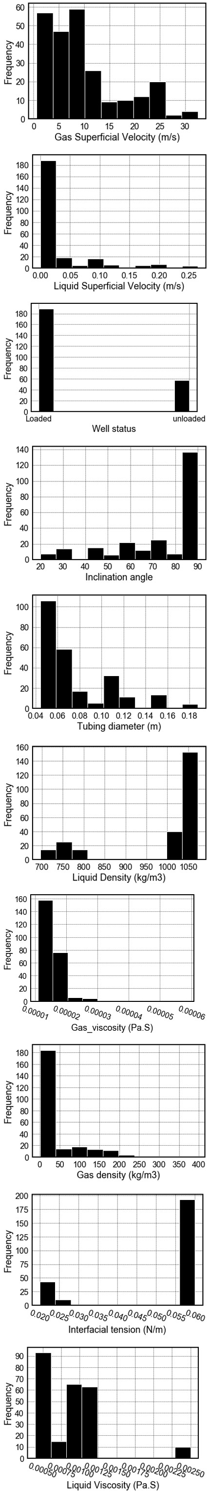
where field engineers measure their fluid properties and rely on to determine the status of the well whether is loaded or not. This explains the high values shown in the plot which also refers to a high-pressure producing well. The interfacial tension plot also indicates that both water and condensate are coproduced with gas.
The total measurements obtained from the data gathered resulted in 246 measurements for both field and lab experiments (196 samples from field studies and 50 samples from lab experiments).
Modelling Method
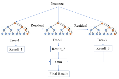
Chen, et al. [20] at the University of Washington, developed XGBoost for the first time and described it as a scalable Machine Learning system for tree boosting. The basis of XGBoost is set on decision trees as the classifier or regressor, including some modifications of the objective function by adding some regularization to limit the over- fitting. An important novelty in the XGBoost is the boosting mechanism introduced, which not only boosts the decision trees but also makes the computation faster than any other ML algorithm. What makes the XGBoost different than Random-Forest and other tree-based algorithms is the architecture that keeps building on previous trees and keeps minimizing the error until it becomes infinitely small (Figure 2). Chen, et al. [20] stated on their paper the mechanism on how the algorithm works by the following example: For a dataset of m features and n number of examples where $$ D = \left\{\left(x _ {i}, y _ {i}\right) \left(\left| D \right| = n, x _ {i} \in \mathbb {R} ^ {m}, y _ {i} \in \mathbb {R}\right), \right. $$
, the output
iy is predicted using K additive functions as follows:
k ∝ ( ) ( )
$$ = \phi \left(x _ {i}\right) = \sum_ {k = 1} ^ {k} f _ {k} \left(x _ {i}\right), f _ {k} \in \mathbb {F} $$
1 , i i k i k k y x f x f φ Here 𝔽 is the space of regression trees, and k is the number of trees in the model. The solution of the model is obtained by minimizing the regularization loss function and by finding the best set of functions to embed in the model:
$$ \mathcal {L} (\phi) = \sum_ {i} l \left(\widehat {y _ {i}}, y _ {i}\right) + \sum_ {k} \Omega \left(f _ {k}\right) $$ where, $$ \Omega (f) = \gamma T + \frac {1}{2} \lambda \omega^ {2} $$ ( ) Here l represents the loss function, or the difference between the predicted output ∝ iy and the actual output iy . Ω measures the complexity of the model and controls the over- fitting of the model. T is the number of leaves of the tree, w is the weight of each leaf.
The term Boosting refers to the process of adding new function f as the model keeps training while working on minimizing the objective function in decision trees. Trees or functions are added as follows:
$$ \mathcal {C} ^ {(t)} = \sum_ {i = 1} ^ {n} l \left(y _ {i}, \hat {y} _ {i} ^ {(t - 1)} + f _ {i} \left(x _ {i}\right)\right) + \Omega \left(f _ {i}\right) $$ ( ) ( ) ( ) ( ) ( ) 1 $$ \mathcal {L} ^ {(t)} = \sum_ {i = 1} ^ {n} l \left(y _ {i}, \hat {y} _ {i} ^ {(t - 1)} + f _ {i} \left(x _ {i}\right)\right) + \Omega () $$
1 , ˆ
( ) ( ) ( )
= + − + + + +
2 2 2 1 2 ∑ ∑ ∑ ∑ ∑ ∑ Λ
g g g i i i i I i I i l split i i i i I i I i l ∈ ∈ ∈ h h h γ λ λ λ L R ∈ ∈ ∈ L R where, ( ) ( ) ( ) 1 ˆ $$ g _ {i} = \partial_ {\hat {y} ^ {(t - 1)}} l \left(y _ {i}, \hat {y} ^ {(t - 1)}\right) $$ ( ) ( ) ( ) 1 1 2 $$ h _ {i} = \partial_ {\hat {y} ^ {(t - 1)}} ^ {2} l \left(y _ {i}, \hat {y} ^ {(t - 1)}\right) $$ Here , i i g h are first and second order gradient statistics on the loss function.
The complete model equations and details can be found in the article by Chen, et al. [20].
As can be seen, the model has multiple parameters, often referred to as hyper parameters that construct a full set of equations to be solved to obtain a final prediction of the critical gas velocity. The model equations are translated to a coded algorithm that trains on the data supplied and then tested to get the best performance. It is worth mentioning that all the coding related to this research was done in Python. This open-source programming language was used to model and tune the model’s hyperparameters to produce the final predictive model. The process of tuning the parameters will be discussed in the next section.
Modelling Approach
The standard field practice is to calculate the critical gas velocity at which liquid loading occurs, using correlations such as Barnea [17]; Luo, et al. [27]; Turner, et al. [9] or transient multiphase flow simulations. This process is done before and after the onset of liquid loading and results in classifying the well as ‘Loaded’ or ‘Unloaded’. Since we are employing Machine Learning to model this problem, the solution provided will contain two parts:
- The first part is a classification problem where a classification model of XGBoost will be developed and compared with the correlations commonly used in literature to see which method better classifies the wells to their correct state.
- The second part is a regression problem where a regression model of XGBoost will be developed to predict a value of a critical gas velocity at which liquid loading occurs, then compare the results of the prediction with the same correlations.
The reason behind this modeling approach is that a correlation or a model may be conservative and predict critical gas velocity values higher than what was observed in the field or the lab leading to wrong interventions, which may cause extra expenses that could have been avoided. In the reverse case, a model could be too optimistic and consistently predict values less than what was observed in the field, which may lead to more damages that could have been avoided. Contemplating this problem, this paper proposes a two-step modeling approach to generate a cost- effective tool that will not only classify the wells as loaded or not but also provide a close approximation of what was observed in the field at the onset of liquid loading.
Since the two steps fall under the Machine Learning modeling, data will be divided randomly with a ratio of 80% training to 20% testing.
Classification problem: This section aims to develop a model that classifies the well to a correct status, whether loaded or not. The first step is to encode the status to an interpretable numeric value; for this purpose, the following coding was considered (Table 1):
| Well status | Status Code |
|---|---|
| Loaded | 1 |
| Unloaded | 0 |
Table 1: Status encoding.
After encoding the well’s status, the first practice is to choose the features to be asserted as inputs for the model. Since the problem being solved is not a purely statistical problem, so it will not be treated as conventional statistical problems where features are selected using technics like recursive features elimination or principal component analysis; rather, the features will be chosen based on previous observations from analytical models such as the liquid film model by Barnea or correlations such as Turner correlation. The reason behind this comes from the engineering perspective of the problem, where each parameter presents specific influence on the problem. Considering the analytical film model by Barnea (Appendix) the following parameters coming from the momentum balance equation are chosen to be inputs for the model (diameter, liquid density, gas density, liquid viscosity, gas viscosity, angle of inclination from horizontal (alpha) and superficial liquid velocity). Considering the model of Turner (Appendix), the interfacial tension is added to the inputs list.
Building an effective classification XGBoost model requires tuning the hyperparameters used inside the model to generate a prediction. To tune the parameters, multiple values should be tested; for that, the Randomized Search technic from Scikit-Learn was used.
RandomizedSearchCV implements a “fit” and a “score” method; it uses a random combination of the hyperparameters from the supplied lists of the values to train and test the model by applying specified cross-validation over the data. Randomized Search chooses the combination of the hyperparameters, which gave a better performance on the testing data. The list of the parameters considered to be tuned is below:
- Number of estimators: this parameter controls the number of decision trees used by the XGBoost. Values list [20, 50, 100, 200, 300, 500, 1000].
- Lambda: this is used to handle the regularization part of XGBoost and avoid overfitting. Values list [0.01,0.1,1].
- Max-depth: the maximum depth of a tree is used to control overfitting as well. More trees depth means that the model is learning relations very specific to a particular sample. Values list [3, 4, 5, 7, 8, 9, 10, 12, 14, 20].
- Gamma: it specifies the minimum loss reduction required to make a split. Values list [0,0.1,0.25,0.5,1].
- The learning rate: it defines the step size shrinkage used in update to prevent overfitting. Values list [0.01,0.05,0. 1,0.2,0.3,0.5,0.6,1].
The final optimized hyperparameters are presented below (Table 2):
| Parameter | Value selected |
| Number-of-estimators | 300 |
| Lambda | 1 |
| Max-depth | 20 |
| Gamma | 0.1 |
| Learning rate | 0.2 |
Table 2: Hyperparameters selected for the XGBoost classifier.
Since the goal is to compare the performance of the model to other correlations in the literature and looking at the fact that the correlations generate a solid value of the critical gas velocity, the following procedure was followed to bring the results to the same page, as was done by Chemmakh, et al. [30] to compare the predicted values by different correlations and the field observation rates as follows: • If the critical rate predicted by the models is bigger than the field rate and the actual status of the well is loaded, the case is labeled “True Loaded TL”.
- If the critical rate predicted by the models is smaller than the field rate and the actual status of the well is loaded, the case is labeled “False Unloaded FU”.
- If the critical rate predicted by the models is bigger than the field rate and the actual status of the well is unloaded, the case is labeled “False Loaded FL”.
- If the critical rate predicted by the models is smaller than the field rate and the actual status of the well is unloaded, the case is labeled “True Unloaded TU”.
The confusion matrix presented in Figure 3 displays the obtained results for the model’s predictions on the testing dataset (50 samples). The confusion matrix is an effective tool to compare the field observations to the predicted ones. Turner’s model, for example, could predict the correct status of the well only in 15 measurements (3 True Loaded well and 12 True Unloaded wells) and misclassified 35 measurements (34 False Unloaded and 1 False Loaded) which could be interpreted as an underprediction of the critical gas velocity leading to very late alert by classifying a well as flowing while it is already loaded or started loading. Similar observation for the model of Belfroid where it performed similarly to Turner’s model. These two models represent the droplet fallback theory models, and as can be seen here, the models did not perform well as aligned with other research article findings naming Luo, et al. [27]; Shekhar, et al. [29]; Veeken, et al. [14]; Cleide Vieira, et al. [38] that stated the Turner’s model or the droplet fallback models tend to underpredict the critical gas velocity and giving late alerts to field engineers to intervene in the wells.
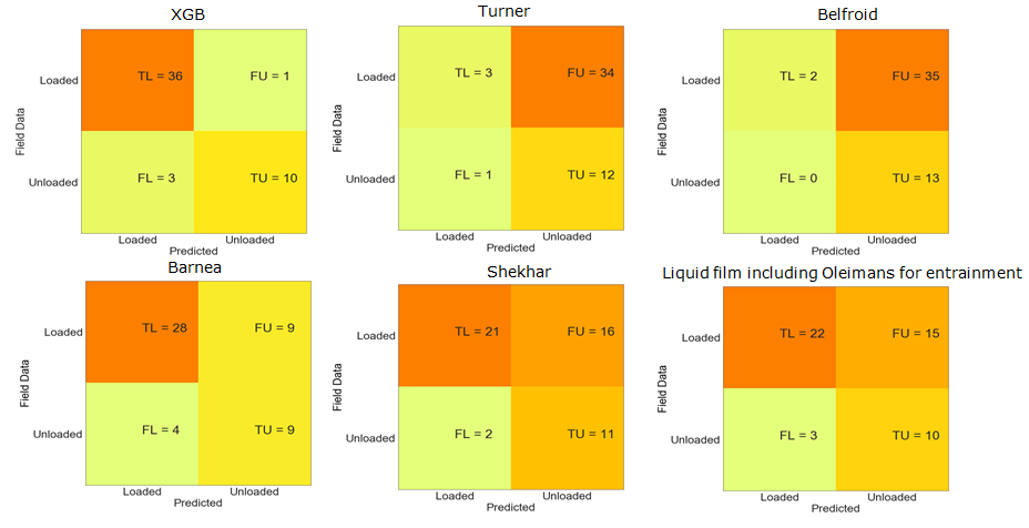
The model of Barnea, on the other hand, performs slightly better by correctly classifying 37 wells/lab measurements as True Loaded (28) or True Unloaded (9); the model of Shekhar also presented better results by correctly classifying 32 wells/lab measurements which is similar to the results of the liquid film model which takes the entrainment into consideration, developed by Chemmakh, et al [30]. The three models representing the liquid film model theory with various modifications, performed better than the droplet entrainment but still underpredicting the results by misclassifying at least 9 wells/lab measurements as False Unloaded which recommends late alert to intervene in the well to reduce liquid loading by considering it as flowing normally while the liquid loading has already started. Contrary, the results obtained from the XGBoost model were reasonably satisfying. The model correctly classified 46 wells/lab measurements from a total of 50 measurements. 36 True loaded and 10 True Unloaded wells show how good the model predictions are by correctly predicting the status of the wells from the supplied inputs. 3 False Loaded cases show that the model overpredicted the results only 3 times. Only 1 False Unloaded case means that the model underpredicted the status of the well only 1 time which reduces the cost of the model predictions by avoiding wrong alerts and missing wells that are loaded and delaying the necessary interventions, making the decisions recommended by XGBoost classifier right on time in most cases in the collected dataset (Table 3).
To further compare the results, the following table presents the metrics often used for classification problems [39, 40]: • Precision: TL TL FL + which is used when the main goal is to be very sure of the prediction. Also, it gives an insight into how many predicted loaded wells are in fact loaded.
• Recall: TL TL FU + is used when predicting loaded wells is a priority as it gives the portion of correctly classified wells among the loaded wells in the field.
- Accuracy: TL TU TL FL TU FU + + + + is the ratio of the correct predictions to the total number of wells. The accuracy may not be the best metric to use when the data is imbalanced (the number of loaded vs. unloaded wells is not even), which is the case for the current data set (37 loaded and 17 unloaded cases). An example would be if a model predicts that all wells are loaded, then it would have an accuracy of 0.74, which is not helpful in the field even though it seems high.
- To overcome the drawbacks of accuracy and to get a balance between precision and recall F1-score is introduced, which takes the harmonic mean of precision and recall.
1 2 F score Precision Recall Precision Recall × = × +
$$ \mathrm {o r} F 1 \mathrm {s c o r e} = \frac {T L}{\left(T L + 0 . 5 \left(F L + F U\right)\right)} $$ Since the F1-score takes both precision and recall into consideration, then any model with a low value of each of them would have as well a low value of F1-score keeping the highest value of F1-score as a reference of which model is the best.
| Names | False Unloaded | False Loaded | True Unloaded | True Loaded | Precision | Recall | Accuracy | F1_Score |
|---|---|---|---|---|---|---|---|---|
| Turner | 34 | 1 | 12 | 3 | 0.75 | 0.081081 | 0.3 | 0.146341 |
| Belfroid | 35 | 0 | 13 | 2 | 1 | 0.054054 | 0.3 | 0.102564 |
| Barnea | 9 | 4 | 9 | 28 | 0.875 | 0.756757 | 0.74 | 0.811594 |
| Shekhar | 16 | 2 | 11 | 21 | 0.913043 | 0.567568 | 0.64 | 0.7 |
| Olimans | 15 | 3 | 10 | 22 | 0.88 | 0.594595 | 0.64 | 0.709677 |
| XGB- Classifier | 1 | 3 | 36 | 10 | 0.923 | 0.972 | 0.92 | 0.947 |
Table 3: Model’s performance metrics.
To assess the results, comparing each metric individually may lead to erroneous results. For instance, looking at the precision alone would choose the model of Belfroid as the best model having a precision of 1, but in fact it could predict only 2 loaded wells from a total of 37. On the other hand, the XGBoost model has a precision of 0.91 but correctly predicted 36 loaded wells from 37. Looking at the recall, the XGBoost has the highest score of 0.972, outperforming the other models clearly. As mentioned before, Recall is used when capturing the loaded wells is a priority. However, it is still not very useful when used alone since a model that predicts all wells are loaded would have a recall of 1 and still not functional. The accuracy metric indicates that XGBoost is the best model, but the result may not be very insightful since the dataset is not symmetric. When using the F1- score, the metric that takes both Precision and Recall into consideration, XGBoost model outperforms all the models with a score of 0.947, followed by the Barnea’s model with a score of 0.81 and the two models derived from the liquid film reversal theory, then comes the models of Turner and Belfroid presenting the droplet fallback theory which again aligns with the results found in Luo, et al. [14]; Shekhar, et al. [29] with only one difference is that the Machine Learning algorithm performed better than all models.
Regression Problem: Predicting the status of the well is crucial but predicting when the well will start loading is equally vital, if not more. For this reason, a model of XGBoost was developed to predict the critical gas velocity. The first step in modeling a regression problem is similar to the classification problem, where the inputs need to be specified. As was done in the previous section, the same inputs were selected based on the observation from previous analytical models and correlations.
Since the model being developed is an XGBoost model, a similar process of optimizing the hyperparameters is integrated into the model. After trying all different combinations, the following parameters were selected and presented the highest performance (Table 4):
| Parameter | Value selected |
|---|---|
| Number-of-estimators | 130 |
| Lambda | 1 |
| Max-depth | 50 |
| Gamma | 1 |
| Learning rate | 0.5 |
Table 4: Hyperparameters selected for the XGBoost regressor.
The model with the best performance was chosen and compared with the different correlations.
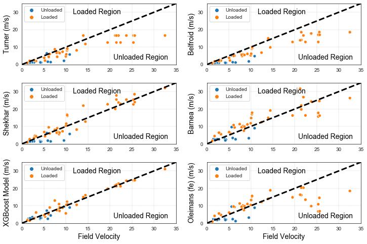
Figure 4 presents the critical gas velocity predicted by the different models compared to the observed critical gas velocity both in field and lab experiments. The results are best when the predictions are on 45 degrees line with the observed critical velocities. The graph showing the models of Turner and Belfroid confirms the previous section’s observation that the models tend to underpredict the critical gas velocity by placing the wells in the unloaded region while they are already loaded. The graph showing the results of XGBoost model predictions demonstrates how close the prediction could be compared to the observed results since most points are either on the 45 degrees line or very close to it. Further comparison of the results requires the introduction of the metrics suitable for regression problems naming: Coefficient of determination R2:
− = − ∑ ∑ n
2 ( ) ( ) y y
predicted true i n
1 =
2 R
2 y y predicted average i
1 = Normalized Root Mean Squared Error NRMSE:
= − = − ∑ n
2 ( ) 1 min y y NRMSE n y y
predicted true i
1 ( ) ( ) true max true
Normalized Mean Absolute Error MAE:
| $NMAE | $\frac{\sum_{i=1}^{n} |y_{predicted} - y_{true}|}{n}$ | $\frac{1}{v - v_0}$ |
|---|---|---|
Table 5: Metrics of model’s performance.
( ) ( ) true max true
The following table sums all the results obtained (Table 5):
| Names | R2 | NMAE | NRMSE |
|---|---|---|---|
| XGB | 0.959851 | 1.203637 | 1.617146 |
| Turner | 0.603237 | 3.766203 | 5.083678 |
| Belfroid | 0.629135 | 3.744506 | 4.914962 |
| Olimans | 0.423974 | 4.056983 | 6.125383 |
| Barnea | 0.733511 | 3.201529 | 4.166311 |
| Shekhar | 0.845328 | 2.433582 | 3.174083 |
Table 6: Metrics of model’s performance.
Comparing R2, XGBoost has the highest score with 0.959, followed by Barnea’s model. Comparing NMAE XGBoost has the lowest value with 0.037, followed by Shekhar’s model with 0.076. Comparing the RMSE, XGBoost has the lowest score with 0.050 confirming the outperformance of the model over all models compared with. The results also prove the previous findings that the liquid film models outperform the droplet fallback models. The model of liquid film model including the entrainment fraction performed the worse and this is also aligning with the conclusions of the work by Chemmakh, et al. [30] that recommended including the entrainment in the Barnea’s liquid film model may not be the best practice.
Results and Discussion
In this research, a Machine Learning method has been utilized to model the problem of the onset of liquid loading in gas wells. The process was divided on two parts:
- A classification problem: here the main goal was to predict the status of the well weather ‘Loaded’ or ‘Unloaded’. In this section the discussion above highlights how the XGBoost could be used as a tool to better predict the status of the wells learning from previous experience and data. The results revealed that XGBoost outperformed all other models and correlations compared with.
- A regression problem: here the goal was to predict when the well will start to load by predicting the critical gas velocity at which the liquids will start to accumulate in the well. The XGBoost model performed better than all other models here as well by predicting the results as close as possible to the field observations with an R2 score of 0.96.
- The only shortcoming of this model is the fact that it is an implicit model that is not quite clear for engineers how to use it. However, with the advancement in the coding skills among engineers, the huge amount of open access resources, and the procedure descried in this paper will give a full roadmap on how to use such an algorithm and predict the onset of liquid loading in gas wells and plan early for the necessary interventions.
References
-
Khetib Y, Rasouli V, Rabiei M, Chellal HAK, Abes A, et al. (2022) Modelling Slugging Induced Flow Instabilities and its Effect on Hydraulic Fractures Integrity in Long Horizontal Wells. 56th U.S. Rock Mechanics/ Geomechanics Symposium, USA.
-
Ouadi H, Mishani S, Rasouli V (2023) Applications of Underbalanced Fishbone Drilling for Improved Recovery and Reduced Carbon Footprint in Unconventional Plays. Petrol Petrochem Eng J 7(1): 1-22.
-
Ansari A, Fathi E, Belyadi F, Takbiri-Borujeni A, Belyadi H (2018) Data-Based Smart Model for Real Time Liquid Loading Diagnostics in Marcellus Shale Via Machine Learning. SPE Canada Unconventional Resources Conference, Canada.
-
Zhang P, Cheng X, Liu R, Yang J, Zheng K (2015) Abnormal Liquid Loading in Gas Wells of the Samandepe Gasfield in Turkmenistan and Countermeasures. Natural Gas Industry B 2(4): 341-346.
-
Ming R, He H (2017) A New Approach for Accurate Prediction of Liquid Loading of Directional Gas Wells in Transition Flow or Turbulent Flow. J Chem 4969765.
-
Djezzar S, Boualam A (2021) Impact of Natural Fractures on the Productivity of Lower Devonian Reservoirs in Reggane Basin, Algeria. 55th U.S. Rock Mechanics/ Geomechanics Symposium, USA.
-
Djezzar S, Boualam A (2020a) Analysis and Modeling of Tight Oil Fractured Reservoir. SEG International Exposition and Annual Meeting.
-
Djezzar S, Boualam A (2020b) Fractures Characterization and Their Impact on the Productivity of Hamra Quartzite Reservoir (Haoud-Berkaoui field, Oued-Mya basin, Algeria). 54th U.S. Rock Mechanics/Geomechanics Symposium, USA.
-
Turner RG, Hubbard MG, Dukler AE (1969) Analysis and Prediction of Minimum Flow Rate for the Continuous Removal of Liquids from Gas Wells. J Pet Technol 21(11): 1475-1482.
-
Belfroid SPC, Schiferli W, Alberts GJN, Veeken CAM, Biezen E (2008) Prediction Onset and Dynamic Behaviour of Liquid Loading Gas Wells. SPE Annual Technical Conference and Exhibition, USA.
-
Coleman SB, Clay HB, McCurdy DG, Norris HL (1991) New Look at Predicting Gas-Well Load-Up. J Pet Technol 43(3): 329-333.
-
Guo B, Ghalambor A, Xu C (2006) A Systematic Approach to Predicting Liquid Loading in Gas Wells. SPE Production & Operations 21(1): 81-88.
-
Nosseir MA, Darwich TA, Sayyouh MH, El Sallaly M (2000) A New Approach for Accurate Prediction of Loading in Gas Wells Under Different Flowing Conditions. SPE Production & Operations 15(4): 241-246.
-
Veeken K, Hu B, Group SPT, Schiferli W (2010) Gas-Well Liquid-Loading-Field-Data Analysis and Multiphase- Flow Modeling. SPE Production & Operations 25(3): 275-284.
-
Wang Z, Guo L, Zhu S, Nydal OJ (2018) Prediction of the Critical Gas Velocity of Liquid Unloading in a Horizontal Gas Well. SPE Journal 23(2): 328-345.
-
Zhou D, Yuan H (2010) A New Model for Predicting Gas- Well Liquid Loading. SPE Production and Operations 25(2): 172-181.
-
Barnea D (1986a) Transition from Annular Flow and from Dispersed Bubble Flow-unified Models for the Whole Range of Pipe Inclinations. Int J Multiph Flow 12(5): 733-744.
-
Adesina F, Damilola FO, Olugbenga F (2013) An Improved Predictive Tool for Liquid Loading in a Gas Well. SPE Nigeria Annual International Conference and Exhibition, Nigeria.
-
Alsaadi Y (2013) Liquid Loading in Highly deviated Gas Wells. Master Thesis, The University of Tulsa, Oklahoma, USA.
-
Chen D, Yao Y, Fu G, Meng H, Xie S (2016) A New Model for Predicting Liquid Loading in Deviated Gas Wells. J Nat Gas Sci Eng 34: 178-184.
-
Fan Y, Pereyra E, Sarica C (2018) Onset of Liquid-Film Reversal in Upward-Inclined Pipes. SPE Journal 23(5): 1630-1647.
-
Liu Y, Luo C, Zhang L, Liu Z, Xie C, et al. (2018) Experimental and modeling studies on the prediction of liquid loading onset in gas wells. J Nat Gas Sci Eng 57: 349-358.
-
van’t Westende JMC, Kemp HK, Belt RJ, Portela LM, Mudde RF, et al. (2007) On the Role of Droplets in Cocurrent Annular and Churn-Annular Pipe Flow. Int J Multiph Flow 33(6): 595-615.
-
Vieira C, Kallager M, Vassmyr M, Forgia NLa, Yang Z (2018) Experimental Investigation of Two-Phase Flow Regime in an Inclined Pipe. 11th North American Conference on Multiphase Production Technology, Canada.
-
Waltrich PJ, Posada C, Martinez J, Falcone G, Barbosa JR (2015) Experimental Investigation on the Prediction of Liquid Loading Initiation in Gas Wells Using a Long Vertical Tube. J Nat Gas Sci Eng 26: 1515-1529.
-
Pagou AL, Wu X, Zhu Z, Peng L (2020) Liquid Film Model for Prediction and Identification of Liquid Loading in Vertical and Inclined Gas Wells. J Pet Sci Engin 188: 106896.
-
Luo S, Kelkar M, Pereyra E, Sarica C (2014) A New Comprehensive Model for Predicting Liquid Loading in Gas Wells. SPE Production and Operations 29(4): 337- 349.
-
Mamudu EEO, Cynthia IB, Samuel ES, Muhammad GBA, Angela OM (2019) Application of Non-Uniform Film Thickness Concept in Predicting Deviated Gas Wells Liquid Loading. MethodsX 6: 2443-2454.
-
Shekhar S, Kelkar M, Hearn WJ, Hain LL (2017) Improved Prediction of Liquid Loading in Gas Wells. SPE Production and Operations 32(4): 539-550.
-
Abderraouf C, Ling K, Olusegun T, Ahmad S (2023) Evaluation of the Onset of Liquid Loading by a Proper Inclusion of Droplet Entrainment. J Energy Resour Technol.
-
Lea J, Nickens H, Wells M (2003) Other Methods to Attack Liquid-Loading Problems. In: Lea J, et al. (Eds.), Gas Well Deliquification, Solution to Gas Well Liquid Loading Problems. Gulf Professional Publishing, pp: 271-282.
-
Gaol AH, Valkó PP (2016) Modeling Wellbore Liquid- Content in Liquid Loading Gas Wells Using the Concept of Characteristic Velocity. SPE Low Perm Symposium, USA.
-
Hu B, Veeken K, Yusuf R (2010) Use of Wellbore- Reservoir Coupled Dynamic Simulation to Evaluate the Cycling Capability of Liquid-Loaded Gas Wells. SPE Annual Technical Conference and Exhibition, Italy.
-
Yusuf R, Veeken K, Hu B (2010) Investigation of Gas Well Liquid Loading with a Transient Multiphase Flow Model. SPE Oil and Gas India Conference and Exhibition, India.
-
Zhang H, Falcone G, Valko P, Teodoriu C, Texas A (2009) Numerical Modeling of Fully-Transient Flow in the Near- Wellbore Region During Liquid Loading in Gas Wells. Latin American and Caribbean Petroleum Engineering Conference, Colombia.
-
Nagoo AS, Kulkarni PM, Arnold C, Dunham M, Sosa J, et al. (2018) A Simple Critical Gas Velocity Equation as Direct Functions of Diameter and Inclination for Horizontal Well Liquid Loading Prediction: Theory and Extensive Field Validation. SPE Artificial Lift Conference and Exhibition – Americas, USA.
-
Vieira C (2020) Modelling and Experimental Study on the Production of Gas Wells with Associated Liquid. NTNU, Norway.
-
Vieira C, Stanko M (2020) Effect of Droplet Entrainment in Liquid Loading Prediction. BHR 19th International Conference on Multiphase Production Technology, France.
-
Laoufi H, Megherbi Z, Zeraibi N, Merzoug A, Ladmia A (2022) Selection of Sand Control Completion Techniques Using Machine Learning. International Geomechanics Symposium, UAE.
-
Mouedden N, Laalam A, Rabiei M, Merzoug A, Ouadi H, et al. (2022) A Screening Methodology Using Fuzzy Logic to Improve the Well Stimulation Candidate Selection. 56th U.S. Rock Mechanics/Geomechanics Symposium, USA.
-
Wallis GB (1969) One-Dimensional Two-Phase Flow. McGraw-Hill.
-
Barnea D (1986b) Transition from Annular Flow and from Dispersed Bubble Flow-unified Models for the Whole Range of Pipe Inclinations. Int J Multiph Flow 12(5): 733-744.
-
Taitel Y, Dukler A (1976) A Model for Predicting Flow Regime Transitions in Horizontal and Near Horizontal Gas-Liquid Flow. AIChE Journal 22(1): 47-55.
- Nigeria’s Vulnerability in the Face of Global Energy Policy
- A Simulation Study of Investigation of Optimum Oil Production Performance by Applying Various Gas Injection Methods in Oil Reservoir
- Characterization of Permo-Triassic Reservoirs through Thermal Maturity Assessment of Westphalian Source Rocks in the Cheshire Basin
- Influence of Microwax on the Rheological and Thermal Behaviour of a Wax Crude Oil
- Real-Time Monitoring and Performance Optimization of Steam Injection in Heavy Oil Reservoirs Using Fiber Optic Sensing and Integrated Predictive Simulation Models
- Rapid On-Site Determination of the Total Petroleum Hydrocarbon Content of Soils by Handheld Fourier Transform Near-Infrared Spectroscopy: Development of a Global, Site- and Scanner- Independent Calibration Model