A Comparative Study on Appraisal of Lithological Boundaries and Litho-Models Using Well Log Data at Bhogpara Oil Field in Assam of NE India
Accurate assessment of bed boundaries at a drill site is a crucial step for reservoir characterization. Generally, the interpreters in oil industries carry out such analysis through expensive softwares based on their experiences and geological knowledge in the study area. However, identifying bed boundaries using traditional interpretation is tedious. In this study, we adopted a synergistic approach of Walsh transform and a bed boundary demarcation technique to discriminate the lithological boundaries in Bhogpara oil field of Assam in NE India. This bed boundary detection technique was tested over self-potential (SP), gamma ray (GR) and laterolog deep resistivity (LLD) logs. Initially, we detected the possible lithological boundaries from GR log variations and hence proposed a lithological model as per the knowledge of traditional log interpretation techniques. Subsequently, Walsh low pass filter was applied to the self-potential (SP), GR and LLD logs to obtain their step function. Afterward, the step functions of logs were processed through the boundary detection algorithm to find out the possible thick and thin beds. Further, bed correlation was made among the Walsh-detected boundaries for the studied wells of the Bhogpara oil field. Finally, a bed boundary model was generated using the boundaries picked from the Walsh-based approach. Our analysis exhibit that the model generated from Walsh boundaries more explicitly envisaged the possible heterogeneity. Traditionally we discriminated the minimum bed thickness of the order of 5.15 m, whereas, from the Walsh-based approach we obtained thin bed of the order of 3.2 m. This proposed bed boundary assessment technique is also helpful in understanding the position of subsurface rock layers as well as possible thick and thin beds when we don’t have any pre-received core information.
Introduction
Discrimination of bed boundary, well correlation and precise measurement of thin beds are the necessary steps involved in reservoir characterization. Generally, the geophysical well log data are used in finding the lithological boundary and petro-physical properties of the formation. Well-log responses are the continuous measurement of petrophysical properties of formation through which the well is drilled. At present, in oil industry spontaneous potential (SP), gamma ray (GR), resistivity (latero-log deep (LLD)), P-wave velocity, bulk density (RHOB) log responses are used for bed boundary detection [1]. In this study only SP, GR, and LLD wire-line log responses having a sampling interval of 0.1 m are used for lithological boundary detection. As well log data register the petrophysical properties of the heterogeneous sub-surface at a particular sampling interval, thus, well log response can be treated as a non-stationary signal [2]. Traditionally, different interpreters use their experience of well logging and geological knowledge of the area. However, different interpreters may sometimes provide dissimilar outcomes from the same data set with same geological condition [3]. According to the quicklook interpretation technique, sudden changes took place in the wireline log data may infer the changes in the lithological layers [4].
Researchers have documented a few non-traditional techniques to interpret rock layer boundaries through the use of wavelet transform-based approaches [2, 5]. However, these wavelet-based techniques are able to discriminate thick lithological layers of the order of 30 m or more. Fang, et al. [6] proposed a technique based on the improved dynamic time warping (IDTW) for stratigraphic correlation using wireline logs. Additionally, in the E&P industry to validate the traditional log interpretation results, core data is not always available for the entire depth section of the drill site, even core recovery is also a difficult task. Though nowadays using the advanced borehole imaging tools like Formation Micro-Scanner (FMS) and Full-bore Formation Micro-Imager (FMI) made by Schlumberger, have the capability to detect bed boundaries in centimeter scales [7]. In petroleum industry, due to cost management, these expensive logs (FMS and FMI) were run only for some specific interest in a particular zone of the reservoir. Therefore, we have to look forward for some unconventional way of interpretation, that may be able to discriminate the lithological boundaries in an automated manner with higher accuracy.
The intention of present study is to find out the plausible thick and thin beds from conventional routine wire log data. Additionally, this technique can provide a general assessment of bed boundary successions of the studied region in more robust manner with less computation time and cost. Numerous techniques and workflows have been recommended and accomplished on bed boundary detection using well log data by applying the Walsh transform, i.e., basically the signal (well log data) passed through Walsh low pass filter [8]. Further researchers used Walsh transform for automated bed boundary detection [9, 10] and log analysis [11]. Walsh transform is also used in other field of geosciences, like, identifying fracture time-frequency analysis of well logs [12], gravity applications [13, 14] and resistivity filtering [15] etc.
In present study, initially the quick look interpretation approach was used on the GR log response to assessed the possible bed boundaries. Subsequently, these beds were correlated among the wells and a traditional lithological model was built-up. In order to obtain the bed boundaries more explicitly, Walsh transform and boundary picking algorithm were applied on available aforesaid wireline logs, as well as a lithological model was proposed on the basis of Walsh picking boundaries.
Walsh Filters and Bed Boundary Detection Algorithm
Walsh transform are a set of complete and orthogonal function of non-sinusoidal waveform. In contrast to sinusoidal waveforms whose amplitudes may assume any value between +1 to -1 [16]. Walsh functions assume only discrete amplitudes that provide the kernel function of the Walsh transform. Because of this special nature of the kernel computation of Walsh transform of a signal is simpler and faster than the Fourier transform. Analogous to the frequency in Fourier analysis, Harmuth [17] has introduced the concept of the generalized frequency in Walsh transform called sequency. Sequency is defined as half of the average number of zero crossing in unit interval (time or space). The unit for sequency is zeros per second (zps). The complete set of Walsh function can be derived through the difference equation as [16],
$$\text{wal}(2k+1) = \left( -1 \right)^{\frac{1}{2}-\frac{1}{4}} \left( \text{wal}(k, 2k+1) + \left( -1 \right)^{\frac{1}{2}-\frac{1}{4}} \text{wal}(k, 2k) \right) \text{for } -\frac{1}{2} \leq x \leq \frac{1}{2} \quad (1)$$
$$= 0 \quad \text{for } -\frac{1}{2} > x > \frac{1}{2} \quad (2)$$
where, $q = 0$ or 1 and $k=0, 1, 2, \ldots$ correspond to the sequence of the Walsh functions. Walsh functions are subdivided into even and odd functions called cosine like Walsh function denoted as Cal (i, t) and sine like Walsh function denoted as Sal (i, t) respectively. i.e.,
$$\text{Cal}(k, x) = \text{wal}(2k, x) \quad (3)$$
and $$\text{Sal}(k, x) = \text{wal}(2k+1, x) \quad (4)$$
A function $f(x)$ defined in the interval $(-1/2, 1/2)$ and satisfying Dirichlet’s conditions can be represented by an infinite series of Walsh functions as [16],
$$f(x) = \sum_{k=0}^{\infty} F(k) \text{wal}(k, x) \quad (5)$$
where,
$$F(k) = \int_{-1/2}^{1/2} f(x) \text{wal}(k, x) \text{d}x \quad (6)$$
For eventually spaced sequence {x(i)} of N number of data sets discrete Walsh Transform is required, is defined as,
1 ,
1 − $$ ) = \frac {1}{N} \sum_ {i = 0} ^ {N - 1} x (i) \operatorname {w a l} (k, i) \tag {7} $$ N ( ) ( ) ( ) i x i wal k i N X k
0 and x(i) can be obtained as,
1 − $$ ) = \sum_ {k = 0} ^ {N - 1} \mathrm {X} (\mathrm {k}) \operatorname {w a l} (\mathrm {k}, \mathrm {i}) \tag {8} $$ N ( ) ( ) ( )
0 , k X k wal k i x i Discrete Walsh transform is mathematically correct, but computational efficiency is found to be less while considering a large data points for analysis due to N2 operations are involved. Thus in practical case, Fast Walsh transform is used that reduces the number of operations to 2 Nlog N . The Walsh transform is found to be superior mathematical tool, having no Gibbs phenomena [18] and no need to choose any special window in time domain. In Walsh filter, the filter coefficients are set to either 0 or 1 [17]. Thus, for Walsh low pass filtering, all sequencies above a certain threshold are multiplied by 0 or 1 [14]. Rock boundary detection was carried out by Walsh low pass versions of well data [8]. Similar algorithms were also applied to detect bed boundary by Maiti and Tiwari [9]. Lanning and Johnson [8] used the depth that corresponds to the initial point of log data as first boundary value. Instead of that it is called as mean boundary value. In present study, the modified methodology has been used. Walsh low pass version of wireline logs, i.e., step functions of the studied logs are considered for modified methodology. Initially, we computed the absolute magnitude difference between present and the mean of the previous values for all previous steps until last boundary was detected. These absolute differences were calculated for all log data simultaneously. Further, each of them was multiplied by a weight value and results are summed up to compute the Walsh pick value. This Walsh pick value is a non-dimensional quantity that measures the amount of change took place simultaneously on all low pass versions of the log data. The term Walsh pick values are compared with another non-dimensional number called “Walsh check” (carefully assigned by the interpreter). This Check is conditioned in a such way that, if Walsh pick is greater or equal to the Walsh check value, then the depth at the beginning of the step is detected as a bed boundary, or else this indicates no new boundary is present in that depth location, and further we go for the repetition of the procedure for the entire studied depth section.
Case Study
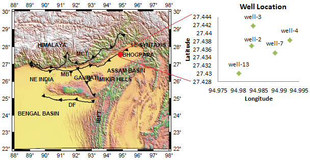
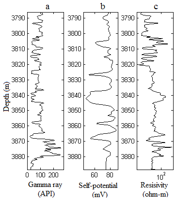
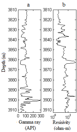
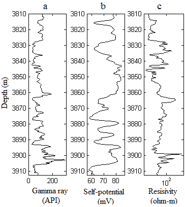
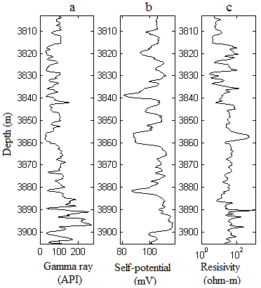
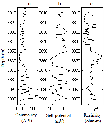
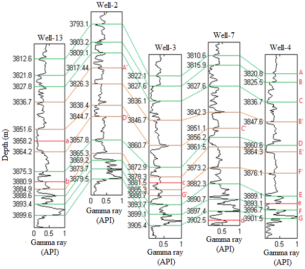
The Assam-Arakan basin is situated in the north-eastern part of India and on the basis of production, this basin is categorized as a Category-I basin. The basin covers an area about 116000 sq. km. The detailed map of this area and well locations are shown in Figure 1. The SP, GR, LLD logs responses are taken for analysis from well-2, well-3, well-4, well-7, well-13 are represented in Figures 2-6, respectively. According to the geology of the Bhogpara area, we selected the depth ranges associated with the Lakadong + Therria formation at the studied wells, as it is the main petroliferous sector of the Bhogpara oil field, belongs to the late Palaeocene epoch.
Bed Boundary Identification and Traditional Model Generation
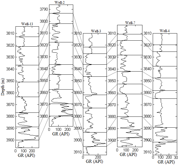
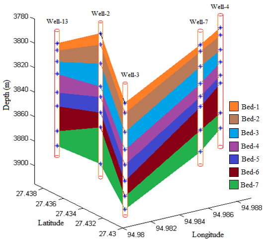
As it is well known that GR log response is very much sensitive to lithology, thus in E&P industry GR log is the preliminary log to use in well correlation. According to quick look interpretation [19, 20] of GR log data, we have deciphered seven beds within the selected depth range of five wells of the Bhogpara oil field, Assam-Arakan basin. Details of bed boundaries are represented in Figure 7 and depth of bed boundaries obtained from different wells are elaborated in Tables 1-5. Further, using the traditionally estimated boundaries, we performed the well correlation task among the studied wells and built-up 3D lithological model (Figure 8). This clearly represents continuation of seven different beds among the studied wells within the working depth range. Further, to achieve better quantitative understanding and for more explicit estimation of the possible thick and thin beds within the selected depth range, the automated Walsh boundary picking algorithm was applied to same log responses.
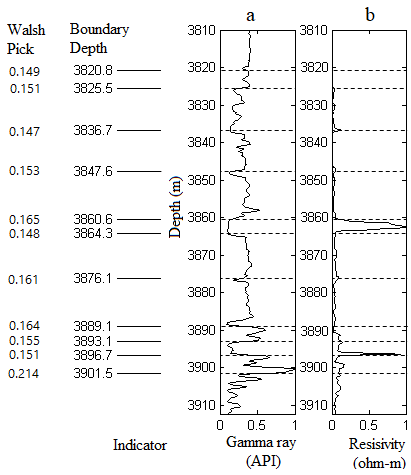
| Step Width (m) | Walsh Pick Value | Walsh Pick Boundary (m) | Conventional Boundary (m) | Remarks (Error in %) | |
|---|---|---|---|---|---|
| 1 | 3.09 | 0.149 | 3820.8 | 3819.61 | 0.0311 |
| 2 | 3.09 | 0.151 | 3825.5 | 3825.42 | 0.002 |
| 3 | 3.09 | 0.147 | 3836.7 | 3837.75 | -0.0274 |
| 4 | 3.09 | 0.153 | 3847.6 | 3847.52 | 0.0021 |
| 5 | 3.09 | 0.165 | 3860.6 | 3858.33 | 0.0587 |
| 6 | 3.09 | 0.148 | 3864.3 | 3865 | -0.0181 |
| 7 | 3.09 | 0.161 | 3876.1 | ||
| 8 | 3.09 | 0.164 | 3889.1 | 3889.42 | -0.0082 |
| 9 | 3.09 | 0.155 | 3893.1 | ||
| 10 | 3.09 | 0.151 | 3896.7 | ||
| 11 | 0.214 | 3901.5 | 3901.76 | -0.0066 |
Table 1: Comparison between Walsh-picked and traditionally-detected boundaries at well-2.
| Step Width (m) | Walsh Pick Value | Walsh Pick Boundary (m) | Conventional Boundary (m) | Remarks (Error in %) | ||
|---|---|---|---|---|---|---|
| 1 | 3.29 | 0.082 | 3793.1 | 3793.02 | 0.0021 | |
| 2 | 3.29 | 0.083 | 3803.2 | 3801.76 | 0.037 | |
| 3 | 3.29 | 0.08 | 3809.1 | |||
| 4 | 3.29 | 0.081 | 3817.44 | 3817.44 | -NIL- | |
| 5 | 3.29 | 0.08 | 3826.3 | |||
| 6 | 3.29 | 0.082 | 3838.4 | 3836.22 | 0.056 | |
| 7 | 3.29 | 0.084 | 3844.7 | 3844.69 | 0.00026 | |
| 8 | 3.29 | 0.082 | 3857.8 | 3857.31 | 0.0127 | |
| 9 | 3.29 | 0.089 | 3865.3 | |||
| 10 | 3.29 | 0.089 | 3869.2 | 3869.39 | -0.0049 | |
| 11 | 3.29 | 0.152 | 3873.7 | |||
| 12 | 3.29 | 0.087 | 3879.5 | |||
| 13 | 3.29 | 3899.66 |
Table 2: Comparison between Walsh-picked and traditionally-detected boundaries at well-3.
| Step Width (m) | Walsh Pick Value | Walsh Pick Boundary (m) | Conventional Boundary (m) | Remarks (Error in %) | |
|---|---|---|---|---|---|
| 1 | 3.09 | 0.063 | 3822.1 | 3821.57 | 0.0138 |
| 2 | 3.09 | 0.072 | 3827.6 | 3827.23 | 0.0097 |
| 3 | 3.09 | 0.071 | 3836.1 | 3836.48 | -0.0099 |
| 4 | 3.09 | 0.071 | 3846.7 | 3846.5 | 0.0052 |
| 5 | 3.09 | 0.073 | 3860.7 | 3861.66 | -0.0248 |
| 7 | 3.09 | 0.071 | 3872.9 | 3872.98 | -0.002 |
| 8 | 3.09 | 0.064 | 3878.3 | ||
| 9 | 3.09 | 0.063 | 3881.5 | ||
| 10 | 3.09 | 0.072 | 3885.3 | ||
| 11 | 3.09 | 0.071 | 3888.7 | ||
| 12 | 3.09 | 0.074 | 3893.7 | 3893.55 | 0.0038 |
| 13 | 3.09 | 0.112 | 3899.1 | ||
| 14 | 3.09 | 0.07 | 3905.4 | 3905.38 | 0.0005 |
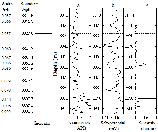
| Sl. No. | Step Width (m) | Walsh Pick Value | Walsh Pick Boundary (m) | Conventional Boundary (m) | Remarks (Error in %) |
| 1 | 3.09 | 0.057 | 3810.6 | 3810.76 | -0.0042 |
| 2 | 3.09 | 0.066 | 3815.9 | 3815.91 | -0.0002 |
| 3 | 3.09 | 0.067 | 3827.6 | 3828.25 | -0.0169 |
| 4 | 3.09 | 0.069 | 3842.3 | 3842.14 | 0.0041 |
| 5 | 3.09 | 0.067 | 3851.1 | ||
| 6 | 3.09 | 3852.67 | |||
| 7 | 3.09 | 0.085 | 3856.2 | ||
| 8 | 3.09 | 0.085 | 3861.5 | 3861.15 | 0.0091 |
| 9 | 3.09 | 0.069 | 3873.2 | ||
| 10 | 3.09 | 0.07 | 3882.3 | 3880.17 | 0.0548 |
| 12 | 3.09 | 0.144 | 3890.7 | ||
| 12 | 3.09 | 0.095 | 3897.4 | 3898.17 | -0.0197 |
| 13 | 3.09 | 0.066 | 3902.5 |
Table 3: Comparison between Walsh-picked and traditionally-detected boundaries at well-4.
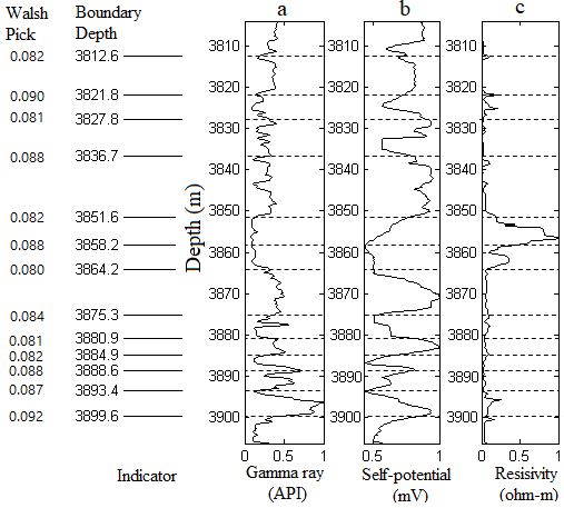
| Step Width (m) | Walsh Pick Value | Walsh Pick Boundary (m) | Conventional Boundary (m) | Remarks (Error in %) | |
|---|---|---|---|---|---|
| 1 | 3.29 | 0.082 | 3812.6 | 3812.82 | -0.0057 |
| 2 | 3.29 | 0.09 | 3821.8 | 3821.063 | 0.0192 |
| 3 | 3.29 | 0.081 | 3827.8 | ||
| 4 | 3.29 | 0.088 | 3836.7 | 3836.73 | -0.0007 |
| 5 | 3.29 | 0.082 | 3851.6 | 3851.142 | 0.0118 |
| 7 | 3.29 | 0.088 | 3858.2 | ||
| 8 | 3.29 | 0.08 | 3864.2 | 3863.47 | 0.0188 |
| 9 | 3.29 | 0.084 | 3875.3 | 3876.83 | -0.0395 |
| 10 | 3.29 | 0.081 | 3880.9 | ||
| 11 | 3.29 | 0.082 | 3884.9 | ||
| 12 | 3.29 | 0.088 | 3888.6 | 3888.91 | -0.0079 |
| 14 | 3.29 | 0.087 | 3893.4 | ||
| 16 | 0.092 | 3899.6 | 3899.98 | -0.0098 |
Table 4: Comparison between Walsh-picked and traditionally-detected boundaries at well-13.
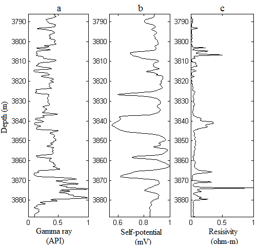
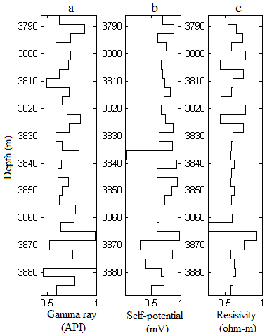
Application of Walsh Transform on Raw Log Data
The aforesaid bed boundary algorithm was applied on the wireline logs to identify the bed boundaries at Bhogpara oil field of Assam-Arakan basin. Initially, we normalized the log responses (GR, SP and LLD) of the studied wells and computed their Walsh low pass version. For an example the normalized the log responses at well-2, and their associated Walsh low pass version are shown in Figure 9 and Figure 10 respectively. According to the limitations of the method, one will not be able to detect bed(s) thinner than the step width of the low pass version of the log response. The step width (is an adjustable quantity) is a function of cut-off sequency that is used in the Walsh low pass filtering operation. As per the methodology applied by Lanning and Johnson [8], cut- off sequency bears inverse relation with step-width of the Walsh low pass data. The quantity step-width (=total band width/width of the low-pass band) is constant, if the cut off sequency is varied from 2N-1+1 to 2N, where N is numbers of data points. In present study, 1024 number of data points are used, and hence the cut off sequency is varied from 4 zero crossing per meter (zpm) to 3 zpm.
As discussed by Lanning and Johnson [8], the Walsh transform is a real number operation, it does not convey any phase information from the input signal. The entire low pass versions of the log data have varied value for every step length. Thus, if the real location of boundary is not exactly situated at the multiple of step length of the Walsh low pass versions, then signal energy corresponding to the transition between two beds will be distributed among the previous and subsequent steps. Therefore, Walsh boundary detection algorithm can identify bed boundaries up to the accuracy of one half of the step length. Lanning and Johnson [8], have given a formula to get the correct depth of boundary, is written as:
$$ B _ {i} = W _ {i} \pm \frac {\Delta S}{2} \tag {9} $$
where, Bi is true location of the ith boundary, Wi Walsh detected boundary and ΔS is step length of the Walsh low pass version. Further in order to get the true location of the boundary, two sets of boundary can be averaged.
$$ B _ {i} = W _ {i} ^ {\prime} \pm \frac {\Delta S}{2} \tag {10} $$
' i W is the final ith boundary detected by un-filtered Walsh method, which leads to the resolution improvement by factor two.
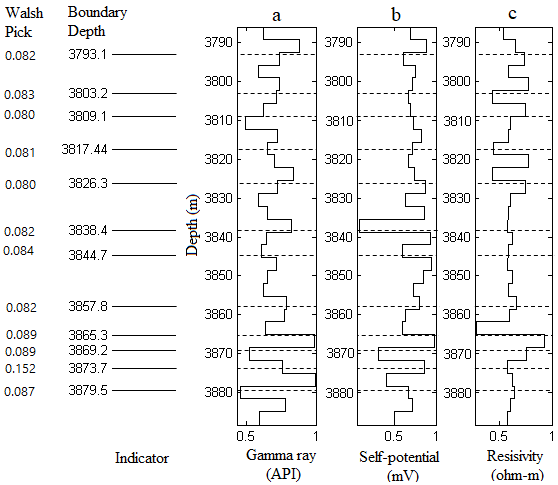
where, In present study, the step width for well-2 and well-13 is 3.29 m, similarly for well-3, well-4, well-7 the step width value is 3.09. In the boundary pick algorithm, equal and/ or different weights have to be assigned to each Walsh low pass version of log data for a particular well, during the data analysis. Here different weights are assigned for different log response in order to achieve required amplification of low passed version log responses, associated to the studied wells. As per the analysis of well-2, weight values assigned to GR, SP, LLD logs are 0.29, 0.32 and 0.39, respectively. Further, details of weights, assigned to the low pass version of studied logs, are represented in Table 6. In accordance with this analysis, the Walsh check value varies from 0.065 to 0.08. For example, according to implemented algorithm, the Walsh picked boundaries obtained from the Walsh low pass version of the wireline logs at well-2 are shown in Figure 11. Here the right column numbers are associated with the boundary depths labelled as “Walsh pick”. Where the pick value is greater than or equal to the “Walsh check” value for that specified depth. Therefore, the Walsh pick is a measure of the depth that is being a boundary.
| Well ID | Log response | Weight value |
|---|---|---|
| Well-2 | GR | 0.29 |
| SP | 0.32 | |
| LLD | 0.39 | |
| Well-3 | GR | 0.27 |
| SP | 0.36 | |
| LLD | 0.37 | |
| Well-4 | GR | 0.33 |
| SP | 0.31 | |
| LLD | 0.36 | |
| Well-7 | GR | 0.28 |
| SP | 0.35 | |
| LLD | 0.37 | |
| Well-13 | GR | 0.3 |
| SP | 0.33 | |
| LLD | 0.37 |
Table 5: Weights assigned to the logs of the wells under study.
Finally, using the aforesaid method, the identified bed boundaries are plotted over the three sets of original log data (GR, SP and LLD) that are associated to well-2, well- 3, well-4, well-7 and well-13 and are shown in the Figures
12-16, respectively. The Walsh transform approached derived bed boundaries are also well corroborated with the conventionally determined bed boundaries. In addition, a few more boundaries are also detected that were very difficult to recognize visually as well as through the conventional techniques. Walsh detected bed boundaries, associated to several wells, are represented in Tables 1-5, respectively.
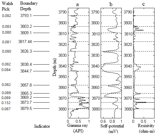
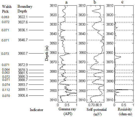
According to this analysis for the well-2 and 13, step length is 3.29 m and the obtained fine bed is of thickness 3.7 m. Further, for well-3, 4 and 7 the step length is 3.09 m and the finest bed thickness obtained as 3.2 m. It is also noted from the last columns of the tables (Table 1, Table 2, Table 3, Table 4 and Table 5) that Walsh picked boundaries are well corroborated with the traditionally interpreted boundaries.
Model Generation Based on the Boundaries Obtained from the Walsh Boundary Picking Technique
As per the un-conventional boundary picking algorithm (Walsh boundary picking algorithm), possible thin beds are obtained from studied wells, that belongs to Bhogpara oil field. Walsh boundary picking technique application leads to estimation of more numbers of thin beds than the traditional quick look interpretation. However, according to the traditional interpretation method only 7 beds are demarcated. In order to map out the bed rock successions more explicitly and precisely for Bhogpara oil field a model is built-up on the basis of Walsh picking boundary technique. The two-dimensional (2D) bed boundary correlation based on the Walsh bed boundary detection technique is represented in Figure 17. Further, in this two-dimensional bed correlation section, we observed a few boundaries that are continuous among all of the studied wells (Well-2, Well-3, Well-4, Well-7, and Well-13), that are named as A, B, C, D, E and F. However, a few boundaries are not continuous among the studied wells, that are named as A′, Bʹ, Cʹ, D′, Eʹ and F′. Moreover, some of the bed boundary exists on a particular well, but found to be absent in neighbor wells, those are named as a, b, c, d and e.
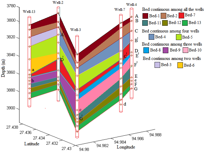
To get a bird’s eye view, we have built the 3-D model based on the Walsh picking boundary procedure. In the 3-D model, the continuation of bed boundary as well as the latitude and longitude of each of the studied wells are represented in Figure 18. It is clearly observed that Bed-1, Bed-2, Bed-7, Bed-11, Bed-12, and Bed-13 are continuous among all the studied wells. However, Bed-4 and Bed-5 are continuous among four wells (Well-2, Well-3, Well-4 and Well-7). Bed-8 and Bed-10 are continuous among three wells (Well-3, Well-4 and Well-7). Bed-9 is also continuous among three wells (Well-13, Well-2 and Well-3). Bed-3 and Bed-6 are continuous among two wells only (Well-13 and Well-2).
Discussion
To identify the rock boundaries in an automated manner, we implemented the modified Walsh based bed boundary detection technique proposed by Maiti and Tiwari [9], which was originally introduced by Lanning and Johnson [8]. We implemented the Walsh based bed boundary detection technique on the wireline logs associated with the Bhogpara oil field of Assam-Arakan basin. Initially, the conventional bed boundaries are demarcated using the GR log data only, afterwards, using these traditionally demarcated boundaries, we computed the 3D lithological model. Further, the Walsh boundary picking technique was applied to the GR, SP and LLD logs to obtain the possible bed boundaries more precisely. It is clearly seen that the Walsh detected boundaries are well corroborated with the conventionally demarcated boundaries in addition to a few thin beds using Walsh transform-based technique. Walsh transform technique has added advantage to the traditional interpretation technique, i.e., it can identify the finest bed that was very difficult to be recognized in traditional interpretation. Therefore, the proposed non-conventional model shows more number of beds and it represents the lithological succession with higher precision as compared to the conventional model. Thus, if this type of non-conventional interpretation is carried out in parallel with the traditional one, we may have less chance of misinterpretation and this approach will be able to generate more accurate lithological model in any study area.
Here we have used only three conventional logs such as gamma ray, laterolog deep resistivity and self-potential logs, However, in addition to the aforesaid logs, oil industry people generally use bulk density, photoelectric factor and neutron porosity logs to find out the rock layers more accurately [1]. Additionally, the self-potential log data is not recorded in marine sediments [4]. Therefore, to interpret rock layer boundaries, researchers must use gamma ray, laterolog deep resistivity, bulk density, neutron porosity and photoelectric factor simultaneously to achieve best and geologically meaningful result.
However, in this technique, the detected bed boundary is ‘weight’ and ‘check value’ dependent and these values are assigned by interpreter. Thus, the number of detected boundaries can be controlled by changing the ‘weight’ and ‘check’ values. Therefore, interpreter must have to choose the ‘weight’ and ‘check’ values in such a way that, at least a few numbers of the Walsh picking boundaries are more or less well corroborated with conventionally interpreted boundaries or the boundaries derived from the core information. Thus, the interpreter has to be careful while choosing the values of ‘weight’ and ‘check’ in order to get geologically meaningful results.
The borehole image logs identify the thin bed in centimeters scale [7], but these are very costly and usually measure specific depth of interest instead of whole depths of a particular well. Therefore, instead of using borehole image logs, Walsh boundary detection techniques can be used for assessing the bed boundary distribution of any reservoir using routine wireline logs.
Conclusions
We have analysed the gamma ray, self-potential and laterolog deep resistivity logs associated with the five wells (well2, well-3, well-4, well-7 and well-13) of Bhogpara oil field in the Assam-Arakan basin. The step length obtained from the Walsh low pass version is 3.29 m for the well- 2 and well-13, and 3.09 m for well-3, well-4 and well- 7, respectively. The Walsh-derived bed boundaries are corroborated with the traditionally estimated boundaries quite accurately. Additionally, the present approach of bed boundary detection could delineate thin beds of the order of ~3 m from the gamma ray, self-potential and laterolog deep resistivity logs. Whereas, the bed boundary, derived through the traditional (quicklook) interpretation of gamma ray, is ~5 m. Therefore, the litho-model derived from the Walsh technique shows finer distribution of rock strata and their continuation throughout the wells under study than the litho-model established based on the bed boundaries derived based on traditional interpretation. We must mention that the number of detected boundaries using Walsh-based approach depends on weights and ‘check’ values. Thus, interpreter should carefully assign the weights and ‘check’ values to achieve geologically meaningful results. Thus, the practical implementation of the Walsh based boundary detection technique to the wireline logs is an efficient, automated and trustworthy technique to demarcate the rock layer boundaries of a hydrocarbon reservoir. Moreover, the Walsh based technique allows multiple logs simultaneously to achieve higher accuracy and hence escapes tedious task involved in traditional or quick-look interpretation. This technique also facilitates the generalized appraisal of distribution of rock layers from conventional logs by avoiding unnecessarily use of expansive image logs. The technique is also one of the robust techniques to find out rock layers based on simultaneous blockiness changes of the logs, when we don’t have any a-priori core information or rock layers.
Acknowledgments
First author is thankful to the Director, Wadia Institute of Himalaya Geology, Dehradun for permission to publish this work. We are grateful to the Oil India Limited (OIL), Duliajan, Assam and GM, Geology and reservoir section of this company, who allowed us to use their well-log data. Our special gratitude to Mr. S. Rath, Former Director (Exploration & Operations), OIL for his kind initiative to support this research with data of OIL. The author also acknowledges the anonymous reviewers for improving the manuscript. KS also acknowledges SERB-DST for providing him with the JC Bose National Fellowship.
References
-
Schlumberger (1989) Log Interpretation Principles/ Applications. Schlumberger Educational Services, Houston.
-
Mukherjee B, Srivhardhan V, Roy PNS (2016) Identification of bed boundary by using wavelet and Fourier transforms. Journal of Applied Geophysics 128: 140-149.
-
Dewan JT (1983) Essentials of Modern Open-Hole Log Interpretation. Penn Well Publishing Company, Tulsa, Oklahoma, USA.
-
Bateman RM (2012) Open hole log analysis and formation evaluation. 2nd(Edn.), Society of Petroleum Engineers, USA.
-
Pan S, Hsieh B, Lu M, Lin Z (2008) Identification of stratigraphic formation interfaces using wavelet and Fourier transforms. Compt & Geosci 34(1): 77-92.
-
Fang H, Lou Y, Zhang B, Xu H, Lu M (2021) Mimicking the process of manual sequence stratigraphy well correlation. Interpretation 9(3): T667-T684.
-
Gaillot P, Brewer T, Pezard P, Yeh EC (2007) Borehole imaging tools- principles and applications. Sci Drill 5: 1-4.
-
Lannin EN, Johnson DM, (1983) Automated identification of rock boundaries: an application of the Walsh transform to geophysical well-log analysis. Geophysics 48(2): 125- 248.
-
Maiti S, Tiwari RK (2005) Automatic detection of lithologic boundaries using the Walsh transform: A case study from the KTB borehole. Compt & Geosci 31(8): 949-955.
-
Mukherjee B, Roy PNS (2016) Comparative Study of Unconventional Tools in Reservoir Characterisation: Case Study from Bhogpara, N-E, India. Journal of Geophysics 37(2): 65-75.
-
Doveton JH (1986) Log analysis of subsurface Geology: Concepts and Computer Methods. Wiley, New York, USA.
-
Jianping Y, Hongpeng Y, Haiyun X (2011) Identifying Fracture by Time-Frequency Analysis of Well Logs. International Conference on Computational and Information Sciences, China, pp: 652-654.
-
Shaw RK, Agarwal BNP, Nandi BK (1998) Walsh spectra of gravity anomalies over some simple sources. Journal of Applied Geophysics 40(4): 179-186.
-
Keating P (1992) Density mapping from gravity data using the Walsh transform. Geophysics 57(4): 522-661.
-
Pal CP (1991) A Walsh Sequency filtration method for integrating the resistivity log and sounding data. Geophysics 56(8): 1140-1295.
-
Beauchamp KG (1975) Walsh Function and their Applications. Academic Press, University of Michigan, USA.
-
Harmuth HF (1968) Sequency filters based on Walsh functions. IEEE Transactions on Electromagnetic Compatibility EMC 10(2): 293-295.
-
Bath M (1974) Spectral analysis in Geophysics. 1st (Edn.), Elsevier, Amsterdam, Netherlands.
-
Serra O (1984) Fundamentals of well-log Interpretation: Acquisition of Logging Data. Elsevier, Amsterdam.
-
Crain ER (1986) The Log Analysis Handbook. Volume 1: Quantitative Log Analysis Methods. Penn Well Publishing Company, Tulsa, Oklahoma.
- Nigeria’s Vulnerability in the Face of Global Energy Policy
- A Simulation Study of Investigation of Optimum Oil Production Performance by Applying Various Gas Injection Methods in Oil Reservoir
- Characterization of Permo-Triassic Reservoirs through Thermal Maturity Assessment of Westphalian Source Rocks in the Cheshire Basin
- Influence of Microwax on the Rheological and Thermal Behaviour of a Wax Crude Oil
- Real-Time Monitoring and Performance Optimization of Steam Injection in Heavy Oil Reservoirs Using Fiber Optic Sensing and Integrated Predictive Simulation Models
- Rapid On-Site Determination of the Total Petroleum Hydrocarbon Content of Soils by Handheld Fourier Transform Near-Infrared Spectroscopy: Development of a Global, Site- and Scanner- Independent Calibration Model