Review of Embedded Discrete Fracture Models: Concepts, Simulation and Pros & Cons
The oil and gas industry faces significant challenges when simulating fractured reservoirs. With the rising cost of hydrocarbons, there is a growing interest in exploiting unconventional reservoirs using hydraulic fracturing technologies. However, unconventional reservoirs typically contain fractured systems at various scales, ranging from nano to kilometer, making it difficult to simulate and predict these reservoirs accurately. Therefore, a rapid and precise method is crucial for this purpose. This paper presents a comprehensive review of the Embedded Discrete Fracture Model (EDFM), a novel approach designed for this purpose. This work begins by reviewing and comparing common methods for simulating naturally and hydraulically fractured reservoirs with EDFM, considering each method's advantages and disadvantages. The concept and formulation of EDFM are then discussed, focusing on adding mass balance equations and making them compatible with reservoir simulators. Additionally, this paper considers the concept and application of non-neighboring connections, which are crucial in simulating fractured reservoirs using EDFM models. This work also highlights the importance of considering changes in the EDFM formulation and simulation when fractures are treated as dynamic systems; failure to do so can lead to significant errors that deviate from actual results. Finally, the disadvantages of EDFM and proposed solutions for enhancing this method are discussed.
Introduction
Fractured hydrocarbon reservoirs pose a challenge in accurately predicting future production and optimizing development plans due to their complexity and heterogeneity. To address this, it is critical to use reservoir simulation and complex fracture system characterization in their development and management [1, 2, 3]. Production rates can show significant early increases followed by a sharp drop when a fracture crosses a production wellbore. Also, Fractures connected to a wellbore can increase production rates compared to reservoirs without such intersections. Fracture characterization typically involves techniques such as Production Logging Tool (PLT), image log, core sample observation, outcrop analog study, and well testing due to the difficulty of directly measuring fracture distribution.
Statistical distribution functions for aperture size, length, and orientation are commonly used to characterize fractures [4, 5]. Fluid flow simulation in fractured reservoirs is critical due to several reasons. Firstly, fractures and matrix exhibit an extreme degree of heterogeneity, which makes it difficult to accurately model reservoirs. Secondly, fractures and matrix vary significantly in scale size which makes it more challenging. Thirdly, it is essential to consider connected corridors that may result in early breakthroughs between wells, linking remote areas of the reservoir. Fourthly, it is crucial to estimate the enhanced productivity accurately due to fracture clusters around the wells. Finally, various recovery mechanisms, such as gravity drainage and imbibition from fractures to matrix, must be taken into account. Accurately considering all these aspects in numerical simulation is computationally challenging. However, doing so may provide a more profound understanding of the system, leading to more effective optimization of field development [6, 7, 8, 9]. The simulation must consider fluid flowing rapidly through low porosity and high permeability fracture networks, a slow mass exchange between the matrix and fractures, and flow in the matrix [10]. The dual continuum approach, which is the state of the art in the oil industry for such reservoirs, distributes matrix and fracture properties in two superimposed corner point grids. Fluid flow between the cells of these grids is driven by a shape factor that represents the relative geometries of the fracture network and matrix block. However, there are limits to this methodology, such as the proper characterization of effective properties for the fracture system and the correct definition of the flow mass transfer coefficient. Consequently, the dual continuum approach may be practical only for highly simplified, regularly distributed fracture networks or reservoirs characterized by diffuse networks with minimal fracture spacing. In other cases, such as reservoirs where fracture corridors and their large-scale connectivity are critical, the dual continuum implementation may be ineffective [11, 12]. The high size contrast between matrix and fracture makes it challenging to model flow behavior in naturally fractured reservoirs (NFRs). Two numerical approaches commonly used to simulate flow in NFRs are continuous and discrete representations. Continuous models, such as the dual- porosity/dual-permeability (DP/DK) approach [13, 14], have been used for decades but suffer from limitations that restrict their ability to accurately represent real fracture networks. DP/DK models assume a constant geometry and properties of the fracture network, and homogenize fracture flow in each simulation block by ignoring connectivity, potentially resulting in unphysical fracture flows between separate reservoir areas. Also, DP/DK models consider matrix and fracture as parallel and continuous systems which requires transfer functions that is dependent of shape factor. This is difficult to be determined for problems involving capillarity, gravity, and fluid systems in which multiple components and phases are present [15]. To address these limitations, discrete fracture-matrix (DFM) methods were developed, which explicitly incorporate fractures as discrete representations. DFM models can simulate complex fracture geometries and accurately account for individual fractures’ effects on fluid flow. Furthermore, the exchange specification between matrix and fracture is relatively straightforward since it directly depends on fracture geometry. Most DFM models use unstructured-grids to account for the geometry and location of fracture systems, though the computational cost can be prohibitive for field-scale applications [16, 17]. The conventional dual porosity/permeability model employs the sugar-cube approximation for matrix and fracture configurations. However, the Effective Discrete Fracture Model (EDFM) does not rely on this approximation. Instead, it directly models the distribution of natural fractures by homogenizing minor fractures and a network of major long fractures. This allows for a more efficient computation compared to the dual permeability and porosity method [4, 17]. The EDFM method uses separate grids for the matrix and the fractures. Fractures are discretized into small control volumes, or fracture segments, by cutting fracture planes with matrix-grid block boundaries. Each fracture segment is explicitly represented as a functional grid block with modified properties [18]. EDFM considers the effect of each fracture explicitly, without requiring the simulation grid to conform to the fracture geometry. This method achieves a compromise between accuracy and efficiency by using standard corner-point grids for the background matrix, along with a discrete representation of the fracture segments that intersect matrix cells. EDFM also employs the concept of transport index to tie the additional computational control volumes for fractures to the matrix [15].
History of NFRs Modeling Methods
NFRs have been modeled using different approaches, which can be broadly categorized into two classes of models: dual-continuum and discrete models. Dual-continuum models have been the traditional and widely used method for simulating NFRs in the industry [16].
Dual-Continuum Models
In the 1960s, Barenblatt, et al. [19] and Warren, et al. [13] introduced the dual-porosity model, also known as the sugar- cube model, for single-phase systems. This model assumes that the rock matrix only serves as fluid storage, while flow occurs entirely in interconnected fractures. Kazemi, et al. [14], Rossen, et al. [20] and Saidi, et al. [21] later extended this approach to multiphase flow and developed dual-porosity simulators. Dual-permeability models were also developed, which allowed for matrix-to-matrix flow. Dual-porosity and dual-permeability models have been widely used in reservoir simulators for naturally fractured reservoirs. However, these models are inadequate to solve fluid-flow problems in complex fractured systems due to the assumptions of uniform fractures, which do not reflect the natural variability of fractures in the simulation. Dual-continuum models are still used today, but they are not accurate for cases where the fracture geometry is complex and asymmetric, such as in unconventional reservoirs. Furthermore, these models cannot explicitly account for the density and orientations of natural fractures, leading to unrealistic results. Multi- continuum models do not distinguish geometrically between matrix, fractures, and fracture intersections [16, 22].
DFN Models
To address the limitations of dual-continuum models, discrete fracture network (DFN) models have been developed. DFN models consider fluid flow and transport through interconnected natural fractures, assuming the matrix is impermeable. These models are particularly useful for fractured rocks where an equivalent continuum model is difficult or not applicable. DFN models can also be used to derive equivalent continuum flow and transport properties for use in faster, upscaled reservoir models. They are suitable for low-permeability and low-porosity fractured media where the flow through the matrix is assumed to be negligible compared to the fractures. Large- scale simulations can be performed using DFN models by approximating the fractured reservoir properties through upscaling and homogenization into equivalent permeability tensors. However, it should be noted that even though DFN models are more precise and efficient, they still require accuracy for simulation purposes, and more advanced methods may need to be developed to meet the demands of complex fractured reservoirs [22, 23].
DFM Models
DFMs (Discrete Fracture Models) represent a newer class of models that have received considerable attention in the last decade for simulating natural fracture networks (NFRs). Compared to dual-continuum and DFN models, DFMs provide more realistic representations of NFRs. Most DFMs rely on unstructured grids to conform to the geometry and location of fracture networks and account explicitly for the effect of individual fractures on fluid flow. Several researchers have developed DFMs based on finite-element methods, including Noorishad, et al. [24], Baca, et al. [25], Jong‐Gyun, et al. [26], and Karimi-Fard, et al. [27], Monteagudo, et al. [28], Fu, et al. [29], Matthai, et al. [30], and Marcondes, et al. [31], Karimi- Fard, et al. [32] and Mallison, et al. [33]. In a DFM model, the fluid resides in both porous matrix and explicit fractures, but the smaller fractures are integrated into the matrix with appropriate upscaling. DFMs are suitable for reservoirs with several natural fractures where only a few dominant fractures contribute to fluid storage and flow [23]. However, generating unstructured grids to conform to the complexity of the fractures in an arbitrary fracture network can be a substantial challenge [34]. Furthermore, the computational cost of using conforming DFMs at the field scale can be prohibitive [15].
EDFM Models
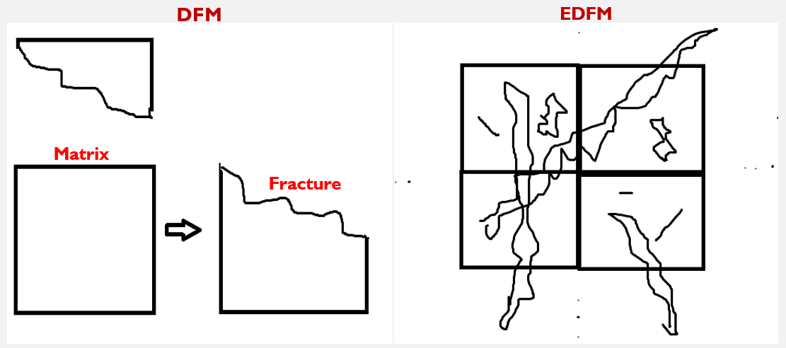
Currently, Embedded Discrete Fracture Models (EDFMs) are the most effective and precise models for simulating NFRs. However, further work is needed to make them fully compatible with industrial and in-house simulators. The EDFM was introduced by Li, et al. [4], which uses a structured grid to represent the matrix and introduces additional fracture control volumes by computing the intersection of fractures with the matrix grid which overcomes the challenges associated with unstructured gridding. In this method, fractures are approximated as vertical planar rectangles with arbitrary orientations in the horizontal plane. EDFM models long fractures in a hierarchical fracture-modeling framework, as most NFRs contain numerous small-scale microfractures and sporadic large-scale macro fractures [35]. Microfractures are shorter than the computational grid dimensions, while macro fractures are field-scale features that extend through multiple grid blocks. Macro fractures have a first- order effect on fluid flow while microfractures are less significant. Consequently, microfractures are homogenized by modifying the effective properties of matrix grid blocks, while large-scale fractures are modeled explicitly by a DFM [34]. In other words, the EDFM uses a hybrid approach in which the dual-porosity model is used for smaller and medium fractures, and DFN is used for larger fractures that are more significant. Fluid flows within the matrix and the fractures are proportionated by the pressure difference between them and are discretized separately, without the need for local grid refinement (LGR) in the vicinity of the fractures which includes high computational cost [22]. Figure 1 indicates the difference between DFM and EDFM model. As it can be seen, fractures can be distributed explicitly through the system of matrix.
Application of NNCs (Non-Neighboring Connections) in EDFM
During the calculation process, complex fractures are discretized into fracture segments based on the interaction between the fracture geometry and structured matrix grid boundaries. Virtual cells are introduced to maintain the properties of the fractures. Fluid flow between the matrix, fractures, and wells can be simulated using NNCs and effective wellbore index within commercial reservoir simulators, as illustrated in Figure 2 [36, 37].
![Figure 2: Computational schematic of NNCs between well, matrix and fracture in reservoir simulator using EDFM [36].](/fulltextimages/10353/fig_2.png)
The EDFM model implements the dual-medium concept from conventional dual-continuum models and accounts for the effect of each fracture explicitly. Unlike conventional approaches, EDFM defines computational fracture control volumes in a separate computational domain instead of the vicinity of matrix grid-blocks. There is no requirement for both grid sizes to be the same since the same grid-block sizes are typically used for both the matrix and fracture domains. Vertical and inclined fractures are discretized both vertically and horizontally by using the cell boundaries of the matrix grid. Regular intersections between a fracture plane and a grid-block result in polygons with three, four, five, or six corners, as depicted in Figure 3. EDFM allows for the explicit incorporation of each fracture’s effect which do not require the simulation grid to conform to the fracture geometry, thus EDFM will lead to a compromise between both accuracy and efficiency, and this is because it enables the use of standard corner-point grids for the background matrix domain [15, 34].
![Figure 3: EDFM allows for the explicit incorporation of each fracture’s effect which do not require the simulation grid to conform to the fracture geometry, thus EDFM will lead to a compromise between both accuracy and efficiency, and this is because it enables the use of standard corner-point grids for the background matrix domain [15,34].](/fulltextimages/10353/fig_3.png)
EDFM separates the fractures and matrix into distinct computational domains, leading to no direct fluid communication between them in the mass-balance equations. To address this, NNCs are defined in EDFM to allow communication between any two grid-blocks in the numerical model. Previous studies have utilized the concept of NNCs in reservoir simulation, such as Dogru, et al. [38], Karimi-Fard, et al. [32] and Mallison, et al. [33] in their DFM approaches. Moinfar, et al. [34] identified three types of NNCs required in EDFM: (1) between a fracture cell and its neighboring matrix grid-block, (2) between two intersecting fractures, where corresponding fracture cells communicate with each other, and (3) between two cells of a fracture which is individual (if needed). This is a result of the fracture arrangement, where grid-blocks need to communicate with each other while they are not computational neighbors in the fracture domain. EDFM requires three types of NNCs in the computational domain to account for the lack of fluid communication between the fractures and the matrix. The first type of NNC is between a fracture segment and the grid- block it is embedded in. The second type of NNC is between the fracture control volumes of intersecting fracture planes in a grid-block. The third type of NNC is between corresponding fracture control volumes of neighboring cells where the fracture segments are not computational neighbors. The intersection line of the fracture plane and the common face of the two-neighboring grid-blocks defines this type of NNC. In order to solve the fluid flow problem in EDFM, a standard finite-volume scheme is used to discretize the equations. According to Sepehrnoori, et al. [18] the transmissibility formulations are written in a form similar to Darcy’s law, where the transmissibility factor depends on several factors including the geometry of the control volumes (i.e. matrix grid-blocks and fracture segments), the relative positions of the control volumes, and the corresponding permeability as:
k A T d = (1)
NNC NNC NNC NNC The transmissibility factor NNC T , permeability NNC k , contact area NNC A , and distance NNC d are all parameters that relate to the NNC in the transmissibility formulations for the EDFM. These parameters are written in a form similar to Darcy’s law, as shown in equation 1. One advantage of this approach is that it simplifies the implementation of the transmissibility equations in a code that involves geometrical calculations.
By adding NNCs to the general form of mass balance equation [34]:
kk V N V x P D q q t φ ξ γ µ = ∂ − ∇ ∇ − ∇ − + = ∂ ∑ ρ ρ ρ
( ) 1 . ( ) 0 p n rj NNC b i b j ij j j i i j j
(2) Where NNC iq is the molar rate of component i exchange through NNCs. This term is mathematically similar to the convection term and is given by:
( ) γ γ ξ µ = = − − − = ∑ ∑
1 1 ( ) NNC p NNC NNC n n j j j j m m rj NNC NNC i m j ij NNC m j j m P D P D k k q A x d (3) The flow potential at a non-neighboring cell is represented by ( )NNC j j m P D γ − , where NNC n is the number of NNCs for a grid-block. NNC m A , NNC m k , and NNC m d are the parameters used to calculate the transmissibility factor between an NNC pair. Represents the area open to flow, NNC m k is the harmonic average of permeability, and NNC m d is the characteristic distance between two control volumes associated with an NNC. To calculate the mobility term in Equation 3, the classical single-point upstream weighting is used. The transmissibility ( ) ( ) / NNC NNC NNC m m m A k d × must be calculated for the three types of NNCs previously described, and the calculation is performed as follows.
When dealing with an NNC between a matrix and a fracture cell, the NNC m A parameter is determined by the fracture surface area within the grid-block. The permeability factor, NNC m k , is the harmonic average of the permeabilities of both the matrix and the fracture and is often like the matrix permeability. In
addition, Li, et al. [4] and Hajibeygi, et al. [39] have proposed that pressure changes linearly in the direction perpendicular to each fracture within a grid-block. They have used the following equation to calculate the average normal distance, NNC m d [34]:
n NNC Vx dv d V = ∫ (4)
The volume element dv , the normal distance nx of the element from the fracture, and the volume of a grid block V are all factors involved in calculating the transmissibility for an NNC between a matrix and a fracture cell. This integral can be computed using numerical methods in a preprocessing code. In the case of an NNC between intersecting fracture cells, a similar approach proposed by Karimi-Fard, et al. [32] is utilized to determine the transmissibility factor, as outlined in Moinfar, et al. [34].
NNC TT k A T T d = + (5)
NNC NNC
1 The transmissibility for an NNC between intersecting fracture cells can be computed using the approach proposed by Karimi-Fard, et al. [32], where int L is the length of the intersection line bounded in a grid-block. Additionally, f ω and fk are the fracture aperture and permeability, respectively, while f d is the average normal distance from the center of fracture subsegments to the intersection line. is calculated by multiplying the fracture aperture by the length of the intersection line. An NNC is required for every pair of intersecting fracture control volumes in a grid-block. However, if two fractures penetrating a grid-block do not intersect within the grid-block, no NNC is necessary [34].
To compute the transmissibility between two cells of an individual fracture, NNC k is set as the fracture permeability, and NNC d is the distance between the centers of two fracture segments. Before running fluid-flow simulations, a preprocessing code should be developed to calculate a list of NNC pairs, fracture cell arrangement, NNC transmissibility, and transmissibility between fracture cells based on the grid structure and fracture planes [40]. Porosity of each fracture control volume is also calculated by dividing the volume of the corresponding fracture segment bounded in a grid-block by the bulk volume of the grid-block. Additionally, the depth of each fracture cell is set equal to the depth of the fracture segment midpoint to consider gravity effects within vertical and nonvertical fractures in the mass-balance equation (Equations 2 and 3). Once the matrix grid and fracture control volumes are entered into a reservoir simulator that allows NNCs, the governing equations for fracture control volumes, similar to those for the matrix medium, are solved using Darcy’s law. Although excessive NNCs may affect the performance of linear solvers in the simulator, this is not typically the case [34]. A fourth type of NNC has been proposed in recent literature to account for the connection between fractures and wells. To calculate the effective wellbore index, a modified Peaceman’s model (see Appendix A) is used [36, 41].
2 W L r r r
w k WI e w e
f f f + = π = (7)
2 2 14.0 , ) / ( ln where fk is the permeability of fracture, f w is the width of fracture, W is the height of fracture-segment and L is the length of fracture-segment [36].
Homogenization of Long Fractures in EDFM
Fracture modeling often involves a stochastic process to generate fractures, which are then categorized by length scales relative to grid-block size. Homogenization is used to calculate the equivalent permeability of each matrix grid- block, with longer, connected fractures that have significant flow impact being explicitly modeled using homogenized media. This method reduces the number of fractures to be explicitly modeled while still capturing small and medium fractures, enhancing computational efficiency. The explicit modeling of a limited number of long fracture systems allows for accurate modeling of dominant flow behavior in naturally fractured reservoirs. A hybrid method that is both numerically efficient and accurate, using planar voids to represent fractures, with flow modeled using two-dimensional Darcy’s law between a pair of parallel plates is proposed by [4]. Fractures in naturally fractured reservoirs often have lengths much larger than the size of the matrix grid-block, but their heights are typically short and equivalent to the grid-block size. To explicitly and efficiently model the transport of fluids between long fractures and matrix grid-blocks, the concept of well bore productivity index (PI) has been applied to derive a transport index [42]. This transport index allows for the formulation of fluid flow as a one-dimensional well-like equation within the fracture and a source/sink term between the fracture and matrix. However, this approach has several limitations, including that fractures are modeled as one- dimensional, not connected, and not allowed to intersect well bores. To overcome these limitations, the classic transport index concept has been extended to include networks of long fractures, model fractures as two-dimensional planes that can penetrate multiple geological layers, and allow fractures to intersect with well bores. This generalized approach leads to a more realistic and complex model of fracture networks, which is more representative of naturally fractured reservoirs [4]. The vertical and horizontal discretization of long fractures is performed by aligning them with the boundaries of the matrix grid-blocks. The flow within these fracture blocks is described by the Darcy equation, which is also applicable to the matrix medium. Therefore, Equations 2-4 can be used to model flow in both fractures and matrix. It is important to note that when applied to fracture flow, these equations represent 2-dimensional flow in the fracture plane, taking into account both the vertical and horizontal directions. The source/sink term in Equations 2-4 can be expanded in a general form as follows:
1 1 1 1 wm wf mf q q q q = + + (8)
The flow of phase i between the well and matrix block is represented by 1 wm q in Eqns. 2-4. Despite the presence of intersecting fractures, Peaceman’s formulation can still be used as an initial estimate for production through the wellbore, but the pressure field may be altered. In addition,
1 wf q represents the flow rate of phase i between the well and fracture in the fracture system and is a new term. The flow rate exchange between the matrix and fracture, represented by 1 mf q , couples the dual continuum media of the matrix and fracture systems.
Homogenization of Short and Medium Fractures in EDFM
Fractures that are very short have a significantly lesser impact on the flow in a grid-block compared to fractures that are similar in length to the grid-block scale. If a fracture is lengthy and cuts through multiple grid-blocks, it is considered as a group of unconnected segments during the calculation of effective permeability. This can lead to underestimation of the effective permeabilities. To overcome this issue, an analytical solution is employed to determine the effective permeability of small fractures. Then, a numerical boundary element method is utilized to calculate the effective permeability for medium-length fractures in each grid-block. The contribution made by short fractures to the effective permeability can be ascertained using the following formula:
( ) ( ) ( )
short i i i N i i i i i i i i short i w w b k w w t t w w t t V λ λ = = ⊗ + ⊗ ∑ ( ) ( ) ( ) ( ) ( ) ( ) ( ) ( ) ( ) ( ) 3 1 2 1 2 1 1 2 1 2 2 1 ( ) , , 12 (9) The fracture is defined by unit tangent vectors ( ) 1 it and ( ) 2 it , while its dimensions in the corresponding tangent vector directions are denoted as ( ) 1 i w and ( ) 2 i w . The operator ⊗is defined as( ) { } i j ij t t t t ⊗ = and V represents the volume of the grid-block. The scalar values given by λ take into account the interaction between the flow of the matrix and the fracture [4].
Transport Index between Matrix and Fracture
In contrast to a well, the pressure gradient around fractures is significantly smaller. Hence, it can be assumed that the pressure around a fracture is distributed linearly. Based on this approximation, the Transport Index for the grid- block, which contains a portion of a long fracture or fracture network, can be calculated. Assuming that the fracture has completely penetrated the vertical thickness of the block, and the grid-block pressure represents the average pressure of the cell, the average normal distance from the fracture can be determined using the following formula:
.n xdS d S ∫ = (10)
Where dS and S are the areal element and area of a grid- block, respectively. Hence, the l-phase flux from matrix to the fracture can be written as:
n b Ak q p f m .) ( . 1 1 1 ∆ λ = (11)
That
f j m i ) (
n p p p − = ∆ d
(12) > < And the transport index becomes:
> < = d n n k A TI . .
(13) Where A is the fracture surface area in the grid-block.
In situations where a fracture has not entirely penetrated the grid-block, it is necessary to first extend the fracture to ensure that it passes through the grid-block. The Transport Index can then be computed using the previously mentioned equation. After calculating the TI for a fully penetrating fracture, it can be assumed that the TI for a partially penetrating fracture is proportional to the length of the fracture within the grid-block, based on a linear relationship [4].
Wells Intersecting Long Fractures
In a reservoir with natural fractures, the productivity of a well significantly relies on whether the wellbore intersects with a broad network of fractures. To address this, a similar approach as in the long fracture model described in the previous section can be adopted, along with a specified pressure condition at the well location. Since the pressure drop inside the fracture is considerably smaller than that between the matrix and the fracture, the transmissibility of the fracture within the block can be expressed as:
f f j f w A k d Λ = (14)
The fracture transmissibility to the wellbore is represented by Ë j , which is dependent on the fracture’s cross-sectional area f A , fracture permeability fk , and the distance between the center of the fracture grid-block and the wellbore f w d . Therefore, the material balance equation can be written with production indices as follows:
( ) ( ) 1 1 1 1 ( ) ( ) i j j j i i w w i w Q b PI b λ λ = Λ Ψ −Ψ + Ψ −Ψ (15) It is assumed that the pressure drop along the fracture within the well block is negligible, and the productivities from the fracture and wellbore can be combined. The Peaceman’s productivity index (PI) formulation can be directly applied under this assumption. However, the pressure field around a wellbore that intersects with a fracture can be significantly different from that of an independent well without fracture intersection, for which Peaceman’s formulation was originally developed. The pressure drop between the well block and wellbore will be considerably smaller due to the contribution from the fracture surfaces within the well block. It should be noted that the primary production will generally occur through the fracture surface, as the fracture transmissibility Ë j is much greater than the productivity index i PI [4].
Black Oil Formulation for Single-Phase Flow in NFRs
Lee, et al. [43] formulation has been extended to develop the fluid flow equations, which can be applied to both matrix medium and long fracture systems and is not limited to a black oil flow model. It should be noted that in this formulation, different phases flow separately. The governing equations for the black oil formulation for oil, water, and gas [30] are used:
( ) [ ] . .( o o o o o o o b S b p g z q t
φ λ ρ ∂ = ∇ ∇ − ∇ − ∂ (16)
( ) [ ] . .( w w w w w w w b S b p g z q t
φ λ ρ ∂ = ∇ ∇ − ∇ − ∂ (17)
( ) [ ] . .( . .( g g s o o
φ λ ρ λ ρ ∂ + = ∇ ∇ − ∇ − + ∇ ∇ − ∇ − ∂
g g g g g s o o o o s o b S R b S b p g z q R b p g z R q t (18) In the simulation, φ represents the media’s porosity, while ob , w b , and gb represent the inverse formation volume factors of the oil, water, and gas phases respectively. The oil, water, and gas phase saturations are denoted by w S , Sg, and Sg respectively, and the simulation time is denoted by t. The specific gravities of the three phases are represented by o λ , w λ , and g λ , while the pressure amounts of each phase are represented by o ρ , w p , and g ρ . The gravity term, vertical distance, and solution gas ratio are represented by g , z, and s R , respectively, and the densities of each phase are represented by o ρ , w ρ , and g ρ . The phase rates are represented by oq , w q , and g q .
Unlike traditional black oil simulation models, equations 16-18 are used to describe both matrix and fracture flow systems, where large fractures are explicitly discretized. The general volumetric flow rate of source/sink, Ql, is determined based on the fracture or matrix system of the transport equation and the presence of a well in the grid block. It’s worth noting that fractures are randomly distributed and can be connected to fractures, matrix, and wells. As a result, the formed Jacobian matrix is not a banded matrix and needs to be solved using a non-banded matrix solver.
Black Oil Formulation for Multi-Phase Flow in NFRs
When multiple phases are flowing simultaneously, the following equations can be used to ensure mass conservation for each phase:
( ) ( ) . fm W b S b u q q t α α α α α α φ ∂= + ∇ = + ∂ (19)
The above equation represents the mass-conservation equations for various phases when they flow simultaneously. The equation includes variables such as porosity φ , saturation Sα , inverse formation volume factor (FVF) bα , and velocity uα of each phase. In addition, the equation includes communication between fracture and matrix domains, denoted by fm qα , which is similar to the flux term, and flow rate for well (source and sink terms), denoted by W qα . The velocities of each phase can be determined using the multiphase extension of Darcy’s Law.
( ) r kk u p g h α α α α ρ µ = − ∇+ ∇ (20)
This paper investigates the immiscible two-phase flow model, with the nonwetting phase being oil (α = o) and the wetting phase being water (α = w). The variables involved are permeability k, viscosity α µ , relative permeability rk α , pressure p, density α ρ , reference density ,ref α ρ , gravitational acceleration g, and height h. The phase saturations are related through the constraint 1 á S ∑ = , and capillary pressure is ignored. It is worth noting that these formulations could be applied to multiphase multicomponent (compositional) fluids, such as those used in thermal EOR methods, but this paper’s scope is limited to the two-phase model. In the case of multiphase fluid, the phase flux becomes:
( ) , , ij ij ij i j F T p p α α λ = − (21)
The phase mobility á ë , where á ë = rk α / α µ , is calculated using single-point upstream weighting, with i and j referring to the aqua and vapor phases. The direction of phase flow is determined by the phase potential difference between neighboring cells [44].
Considering Fracture as Dynamic Phenomena
In simulations of naturally fractured reservoirs, fracture properties are typically treated as static parameters, but to accurately model production, dynamic behavior must be included in a discrete fracture model [45]. Recent studies have shown that pressure-dependent fracture properties have a significant impact on hydrocarbon recovery, with fracture deformation caused by changes in effective stress playing a key role. Pressure depletion can greatly reduce the conductivity of hydraulic fractures, and production or injection activities can induce rock deformations through changes in pore pressure. Changes in pore pressure can also significantly affect the fluid flow characteristics of reservoir rocks, including permeability and pore compressibility. In fractured media, geomechanically effects on fluid flow are particularly important due to the presence of fissures that may be more sensitive to stress changes than the surrounding rock matrix [16]. In Moinfar, et al. [4] proposed a novel approach to model the impact of stress regime on fluid flow in a 3D discrete fracture network. Their coupled geomechanics-EDFM approach considered the non-linear Barton-Bandis joint model to represent normal deformation of natural fractures and accounted for the effect of pressure depletion on fracture conductivity. The simulations revealed that the effect of these on production strongly depends on parameters that control the deformation behavior of fractures. It is also found that creating high-conductivity fractures during stimulation treatment of reservoirs with low permeability can mitigate the adverse effect of hydraulic fracture closure. Furthermore, this approach did not affect the computational performance of EDFM. To capture the dynamic behavior of fractures in EDFM, stress or pressure-dependent empirical models can be used as a simplified approach since a fully coupled fluid flow and geo-mechanic model is very complex and computationally expensive. However, such models neglect important factors like matrix geomechanics and fracture shear deformation. Additionally, the effect of shear stress on fracture conductivity is not well understood, and the impact of fractures and production on local stress changes should be considered to reach more realistic simulations. In other words, fully coupled geomechanics- flow simulations can handle these effects more accurately, but they are computationally expensive and complex. More information regarding this research can be found in Li, et al. [4]. Xu, et al. [18] introduced a new formulation for modeling the dynamic behavior of fractures in numerical simulations. The new formulations, presented in Table 1, are similar in form to traditional transmissibility equations, which mean they can be easily integrated into existing simulators without needing major modifications. Using these new formulations, fractures can be treated as control volumes and the connections between fractures and matrix grid-blocks can be handled in the same way as regular connections. Table 1 summarizes the required equivalent parameters in the modified formulations. Because the transmissibility factors for non-neighboring connections are linked with grid-block permeability, any changes in permeability will be reflected in the modified transmissibility factors. This feature makes it convenient to simulate dynamic processes related to fractures.
| NNC Type | Type of Control Volumes | Contact Area | Equivalent Distance to Matrix | Equivalent Distance to Fracture |
|---|---|---|---|---|
| Type 1 | Matrix grid block and fracture segment | 2A f | k d m f −m n.(k.n) | W f 2 |
| Type 2 | Fracture segments | A c | d seg1 | d seg2 |
| Type 3 | Fracture segments | W L f int | W f d f 1 W f1 | W f d f2 W f2 |
Table1: Formulation for modeling the dynamic behavior of fractures in numerical simulations [18].
Disadvantages of EDFM Models
EDFM may lead to significant errors in multiphase displacement processes because it cannot accurately capture the proper flux distribution through a fracture. In Figure 4, a comparison is made between EDFM and a realistic flow scenario. If a water front moves from right to left, in the realistic process, water will initially enter the matrix cell m2 and then flow into the fracture, where the flux is divided into two parts: along and across the fracture. However, in EDFM, the fracture behaves as a sink term in m2, causing a large portion of the injected fluid to enter the fracture and creating an unrealistic flux distribution, leading to a lower saturation value of m2. The flux across the surface between m1 and m2 decreases because the phase mobility is evaluated at the upstream cell m2. In short, the flow through the fracture in the realistic process should always be from one side to the other. However, EDFM cannot calculate the flux on both sides separately, resulting in fluid preferentially flowing along the fracture [15].
![Figure 4: Comparison of the fluid flow in a fracture in EDFM and the realistic scenario [15].](/fulltextimages/10353/fig_4.png)
When using EDFM, fluids tend to flow more rapidly along a fracture than across it, which can lead to inaccuracies in multiphase displacement processes. EDFM is most suitable for single-well depletion and injection processes where fluids flow simultaneously in and out of fractures. EDFM’s fracture-matrix transfer functions can precisely calculate net fluxes in a fracture considering the fracture only acts as a single source or sink term. According to Jiang, et al. [15], large errors from EDFM are only likely to occur when there are flow field asymmetries or anisotropies around fractures. To address the limitations of EDFM, one potential solution is the use of pEDFM. This method, developed by Tene, et al. [46], is a projection-based extension of EDFM that can effectively overcome the restrictions of the original approach. Specifically, EDFM is not appropriate when fracture permeability is lower than that of the matrix. To solve this issue, pEDFM is designed to accommodate a range of permeabilities. One key advantage of pEDFM is its ability to capture fluxes on both sides of a fracture separately, a limitation of EDFM. The projection concept in pEDFM was initially introduced to address the issue of flow barriers [15].
![Figure 5: Comparison of the fluid flow through a fracture in pEDFM and the realistic scenario [15].](/fulltextimages/10353/fig_5.png)
Figure 5 illustrates a comparison between pEDFM and the physical flow scenario, demonstrating the improved accuracy of pEDFM. In contrast to EDFM, the flow sequence in pEDFM is directed from the fracture to m2 and then to m1, overcoming the limitation of EDFM and capturing separate fluxes on either side of the fracture [15, 47].
More information for methodology and formulations of the pEDFM method can be found in [15]. To address the limitations of EDFM mentioned earlier, the green function method (GEM) can be utilized as an alternative solution. While the original EDFM only considers geometrical properties when computing the interflux conductivity between matrix grids and discrete fracture elements, this approach does not fully align with physical reality. The boundary element method (BEM) could be a viable option to address this issue, but the original BEM is not effective in strongly heterogeneous reservoirs. Thus, the development of a numerical approach to capture transient mass transfer in heterogeneous fractured porous media is crucial. The GEM, a variant of BEM, is capable of effectively handling nonlinear problems in such media. The original GEM proposed by Taigbenu, et al. [48] involves meshing the calculation domain with polygonal cells, with cell vertices treated as unknown nodes [49, 50] (Figures 6-8).
![Figure 6: Schematic of EDFM concept [48].](/fulltextimages/10353/fig_6.png)
![Figure 7: The triangular schematic of a cell for the novel GEM of double nodes of pressure and flux [48].](/fulltextimages/10353/fig_7.png)
![Figure 8: The GEM’s coupling process based on double nodes of pressure and flux [48].](/fulltextimages/10353/fig_8.png)
The early-time results clearly demonstrate that the modified EDFM, utilizing the novel GEM method, outperforms the original EDFM when compared to tNavigator®. This is due to the ability of the GEM method to accurately model the transient mass transfer between fracture elements and local triangle matrix grids, which overcomes the limitations of the linear flow approximation used in the original EDFM. The modified EDFM shows higher precision and robustness, indicating that it is a more reliable method for modeling fractured porous media [48].
Weijermars, et al. [22] proposed an alternative method called Complex Analysis Methods (CAM) to overcome the limitations of EDFM. CAM is an analytical model that accurately models and visualizes flow in various naturally fractured reservoirs. One significant advantage of the CAM model is that it can solve flow equations without any gridding, which makes it computationally efficient and able to model heterogeneous reservoirs with numerous discrete fractures.
This is very useful when modeling flow in unconventional reservoirs consisting many hydraulic and natural fractures. CAM particle paths were found to closely match those obtained by independent methods, such as Eclipse (Figure 9). Overall, CAM provides a low computational load solution with high resolution for modeling flow in naturally fractured reservoirs. It is important to note that while EDFM and CAM have different assumptions and modeling approaches, both methods aim to accurately model and simulate flow in naturally fractured reservoirs. EDFM assumes a dual continuum model and assigns pseudo permeability to fractures based on aperture, while CAM uses an extension of Darcy flow assumption with a flux strength to scale permeability. Additionally, while EDFM uses Dirichlet boundary conditions with constant pressure rate, CAM inputs both velocity and flux with pressure being a consequence. Thus, selecting an appropriate method will depend on the specific needs and aims of the simulation, and both EDFM and CAM offer unique advantages and limitations [51].
![Figure 9: (a) shows the fracture geometry, and (b) indicates Flow paths generated with EDFM and uniform pressure at the left-hand boundary which is normalized using the right-hand boundary held at zero pressure [22].](/fulltextimages/10353/fig_9.png)
Discussion
Dual-continuum models, DFN models, DFM models, and EDFM models are all modeling techniques used to simulate fluid flow and transport in fractured reservoirs. Dual- continuum models were introduced in the 1960s and assume that flow occurs entirely in interconnected fractures, with the rock matrix only serving as fluid storage. These models are inadequate for solving fluid-flow problems in complex fractured systems due to the assumptions of uniform fractures and cannot explicitly account for the density and orientations of natural fractures. To address the limitations of dual-continuum models, discrete fracture network (DFN) models were developed. DFN models consider fluid flow and transport through interconnected natural fractures, assuming the matrix is impermeable. DFN models can be used to derive equivalent continuum flow and transport properties for use in faster, upscaled reservoir models. DFM models represent a newer class of models that provide more realistic representations of natural fracture networks (NFRs). Most DFMs rely on unstructured grids to conform to the geometry and location of fracture networks and account explicitly for the effect of individual fractures on fluid flow. In a DFM model, the fluid resides in both porous matrix and explicit fractures, but the smaller fractures are integrated into the matrix with appropriate upscaling. Currently, Embedded Discrete Fracture Models (EDFMs) are the most effective and precise models for simulating NFRs. EDFMs use a structured grid to represent the matrix and introduce additional fracture control volumes by computing the intersection of fractures with the matrix grid, which overcomes the challenges associated with unstructured gridding. EDFMs
use a hybrid approach in which the dual-porosity model is used for smaller and medium fractures, and DFN is used for larger fractures that are more significant. It is important to note that while these models are more precise and efficient, they still require accuracy for simulation purposes, and more advanced methods may need to be developed to meet the demands of complex fractured reservoirs.
Conclusion
- With the recent increased demand for hydrocarbon products, exploitation of unconventional reservoirs that mostly contain fractured systems or require hydraulic fracturing to enhance production is critical.
- Current mostly used methods to simulate fractured hydrocarbon systems in industry like dual-continuum and LGR methods cannot deliver the required accuracy and usually involve computational cost. Dual-continuum models are computationally efficient but not accurate enough while LGR is highly accurate but requires a lot of time to reach the results. EDFM models have the time efficiency of dual-continuum models, and they are much more accurate than dual-continuum models.
- Possible and efficient formulations that make EDFM compatible with reservoir simulator have been reviewed. These formulations in conjunction with NNCs can be easily implemented in mass balance equations and fed to simulators.
- Simulation with EDFM with considering fractured systems as dynamic systems have been also reviewed. The formulation should be changed because it can lead to huge errors that are far from realistic results.
- Finally, some deficiencies of EDFM models like their inability to capture flooding recovery techniques like water and CO2 flooding were also discussed. Additionally, some post-developed methods like projection based EDFM were also reviewed that can obviate EDFM incapabilities.
References
-
Kim H, Onishi T, Chen H, Datta-Gupt A (2021) Parameterization of embedded discrete fracture models (EDFM) for efficient history matching of fractured reservoirs. Journal of Petroleum Science and Engineerin 204: 108681.
-
Liming Z, Cui C, Xiaopeng M, Sun Z, Liu F, et al. (2019) A fractal discrete fracture network model for history matching of naturally fractured reservoirs. Fractals 27(1): 1940008.
-
Nader G, Hejri S, Sajedian A, Rasaei MR (2015) Consistent porosity–permeability modeling, reservoir rock typing and hydraulic flow unitization in a giant carbonate reservoir. Journal of Petroleum Science and Engineering 131: 58-69.
-
Li L, Lee SH (2008) Efficient field-scale simulation of black oil in a naturally fractured reservoir through discrete fracture networks and homogenized media. SPE Reservoir Evaluation and Engineering 11(4): 750-758.
-
Liyong L, Lee SH (2008) Efficient field-scale simulation of black oil in a naturally fractured reservoir through discrete fracture networks and homogenized media. SPE Reservoir evaluation & engineering 11(4): 750-758.
-
Panfili P, Cominelli A (2014) Simulation of miscible gas injection in a fractured carbonate reservoir using an embedded discrete fracture model. Society of Petroleum Engineers 3: 1632-1652.
-
Mohammed YA, Bouchaala F, Bouzidi Y, Sultan A, Takougang EMT, et al. (2021) Integrated fracture characterization of thamama reservoirs in Abu Dhabi oil field, United Arab Emirates. SPE Reservoir Evaluation & Engineering 24(4): 708-720.
-
Mohsen E, Sajedian A (2010) Use of fuzzy logic for predicting two-phase inflow performance relationship of horizontal oil wells. Trinidad and Tobago Energy Resources Conference, Spain.
-
Sajedian A, Ebrahimi M, Jamialahmadi M (2012) Two- phase inflow performance relationship prediction using two artificial intelligence techniques: Multi-layer perceptron versus genetic programming. Petroleum science and technology 30(16): 1725-1736.
-
Ahmad ASA, Gosselin OR (2008) Matrix-fracture transfer function in dual-medium flow simulation: Review, comparison, and validation. Europec/EAGE conference and exhibition, Italy.
-
Wayne N, Schechter DS, Laird B (2006) Naturally fractured reservoir characterization. Softcover, San Ramon, USA, pp: 115.
-
Rafuqul MI, Hossain ME, Moussavizadegan SH, Mustafiz S, Abou-Kassem JH, et al. (2016) Advanced petroleum reservoir simulation: Towards developing reservoir emulators. 2nd(Edn.), John Wiley & Sons, pp: 592.
-
Warren JE, Root PJI (1963) The behavior of naturally fractured reservoirs. Society of Petroleum Engineers Journal 3(3): 245-255.
-
Kazemi H, Merrill LS, Porterfield KL, Zeman PR (1976) Numerical simulation of water-oil flow in naturally fractured reservoirs. Society of Petroleum Engineers Journal 16(6): 317-326.
-
Jiang J, Younis RM (2017) An improved projection- based embedded discrete fracture model (pEDFM) for multiphase flow in fractured reservoirs. Advances in Water Resources 109: 267-289.
-
Moinfar A, Sepehrnoori K, Johns RT, Varavei A (2013) Coupled geomechanics and flow simulation for an embedded discrete fracture model. Society of Petroleum Engineers 2: 1238-1250.
-
Hematpur H, Abdollahi R, Rostami S, Haghighi M, Blunt MJ, et al. (2023) Review of underground hydrogen storage: Concepts and challenges. Advances in Geo- Energy Research 7(2): 111-131.
-
Xu Y, Yu W, Sepehrnoori K (2019) Modeling dynamic behaviors of complex fractures in conventional reservoir simulators. SPE Reservoir Evaluation and Engineering 22(3): 1110-1130.
-
Barenblatt GI (1962) The mathematical theory of equilibrium cracks in brittle fracture. Advances in applied mechanics 7: 55-129.
-
Rossen RH, Shen EIC (1989) Simulation of gas/oil drainage and water/oil imbibition in naturally fractured reservoirs. SPE Reservoir Engineering 4(4): 464-470.
-
Saidi AM (1983) Simulation of naturally fractured reservoirs. SPE Reservoir Simulation Symposium, USA.
-
Khanal A, Weijermars R (2020) Comparison of Flow Solutions for Naturally Fractured Reservoirs Using Complex Analysis Methods (CAM) and Embedded Discrete Fracture Models (EDFM): Fundamental Design Differences and Improved Scaling Method. Geofluids pp: 8838540.
-
Prince AN, Javadpour F (2012) Dual-continuum modeling of shale and tight gas reservoirs.” SPE annual technical conference and exhibition, USA.
-
Jahan N, Mehran M (1982) An upstream finite element method for solution of transient transport equation in fractured porous media. Water Resources Research 18(3): 588-596.
-
Baca RG, Arnett RC, Langford DW (1984) Modelling fluid flow in fractured‐porous rock masses by finite‐element techniques. International Journal for Numerical Methods in Fluids 4(4): 337-348.
-
Jong‐Gyun K, Deo MD (2000) Finite element, discrete‐ fracture model for multiphase flow in porous media. AIChE Journal 46(6): 1120-1130.
-
Karimi-Fard M, Firoozabadi A (2003) Numerical simulation of water injection in fractured media using the discrete-fracture model and the Galerkin method. SPE Reservoir Evaluation & Engineering 6(2): 117-126.
-
Monteagudo JEP, Firoozabadi A (2004) Control‐ volume method for numerical simulation of two‐phase immiscible flow in two‐and three‐dimensional discrete‐ fractured media. Water resources research 40(7).
-
Michael FC, Glover FW, April J (2005) Simulation optimization: a review, new developments, and applications. Proceedings of the Winter Simulation Conference, USA.
-
Matthäi SK, Geiger S, Roberts SG, Paluszny A, Belayneh M, et al. (2007) Numerical simulation of multi-phase fluid flow in structurally complex reservoirs. Geological Society, London, Special Publications 292(1): 405-429.
-
Marcondes RA, Sanchez TG, Kii MA, Ono CR, Buchpiguel CA, et al. (2010) Repetitive transcranial magnetic stimulation improve tinnitus in normal hearing patients: a double‐blind controlled, clinical and neuroimaging outcome study. Eur J Neurol 17(1): 38-44.
-
Karimi-Fard M, Durlofsky LJ, Aziz K (2004) An efficient discrete-fracture model applicable for general-purpose reservoir simulators. SPE journal 9(2): 227-236.
-
Kok-Thye L, Mun-Hong H, Mallison B (2009) A next- generation reservoir simulator as an enabling technology for a complex discrete fracture modeling workflow. SPE annual technical conference and exhibition, USA.
-
Moinfar A, Varavei A, Sepehrnoori K, Johns RT (2014) Development of an efficient embedded discrete fracture model for 3D compositional reservoir simulation in fractured reservoirs. SPE Journal 19(2): 289-303.
-
Hadi H, Karvounis D, Jenny P (2011) A hierarchical fracture model for the iterative multiscale finite volume method. Journal of Computational Physics 230(24): 8729-8743.
-
Xu F, Yu W, Li X, Miao J, Zhao G, et al. (2018) A fast EDFM method for Production simulation of complex fractures in naturally fractured reservoirs. SPE Eastern Regional Meeting, USA.
-
Wei Y, Xu, Y, Weijermars R, Wu K, Sepehrnoori K, et al. (2017) Impact of well interference on shale oil production performance: a numerical model for analyzing pressure response of fracture hits with complex geometries. SPE hydraulic fracturing technology conference and exhibition, USA.
-
Larry FSK, Dogru AH (2008) Parallel unstructured-solver methods for simulation of complex giant reservoirs. SPE Journal 13(4): 440-446.
-
Hadi H, Karvounis D, Jenny P (2011) A hierarchical fracture model for the iterative multiscale finite volume method. Journal of Computational Physics 230(24): 8729-8743.
-
Wei Y, Xu, Y, Weijermars R, Wu K, Sepehrnoori K, et al. (2018) A numerical model for simulating pressure response of well interference and well performance in tight oil reservoirs with complex–fracture geometries using the fast embedded–discrete–fracture–model method. SPE Reservoir Evaluation & Engineering 21(2): 489-502.
-
Morteza B, Esmailpour K, Refahati N (2023) Feasibility study and thermoeconomic analysis of cooling and heating systems using soil for a residential and greenhouse building. arXiv preprint, pp: 1-13.
-
Liyong L, Lee SH (2008) Efficient field-scale simulation of black oil in a naturally fractured reservoir through discrete fracture networks and homogenized media. SPE Reservoir evaluation & engineering 11(4): 750-758.
-
Han JL, Lee SY (2001) Heat transfer correlation for boiling flows in small rectangular horizontal channels with low aspect ratios. International Journal of Multiphase Flow 27(12): 2043-2062.
-
Jiamin J, Younis RM (2017) An improved projection- based embedded discrete fracture model (pEDFM) for multiphase flow in fractured reservoirs. Advances in water resources 109: 267-289.
-
Hugo A, Lacentre P, Zapata T, Monte AD, Dzelalija F, et al. (2004) Dynamic behavior of discrete fracture network (DFN) models. SPE International Petroleum Conference, Mexico.
-
Matei T, Sebastian BMB, Al-Kobaisi MS, Hajibeygi H (2017) Projection-based embedded discrete fracture model (pEDFM). Advances in Water Resources 105: 205- 216.
-
Jiamin J, Younis RM (2017) An improved projection- based embedded discrete fracture model (pEDFM) for multiphase flow in fractured reservoirs. Advances in water resources 109: 267-289.
-
Akpofure TE (1995) The Green element method. International Journal for Numerical Methods in Engineering 38(13): 2241-2263.
-
Cheng L, Du X, Cao R, Wang Z, Shi J, et al. (2021) A Coupled Novel Green Element and Embedded Discrete Fracture Model for Simulation of Fluid Flow in Fractured Reservoir. Geofluids pp: 9910424.
-
Cheng L, Xulin D, Xiang R, Renyi C, Pin J, et al. (2022) A numerical simulation approach for embedded discrete fracture model coupled Green element method based on two sets of nodes. Chinese Journal of Theoretical and Applied Mechanics 54(10): 2892-2903.
-
Aaditya K, Weijermars R (2020) Comparison of flow solutions for naturally fractured reservoirs using Complex Analysis Methods (CAM) and Embedded Discrete Fracture Models (EDFM): Fundamental design differences and improved scaling method. Geofluids pp: 1-20.
-
Donald PW (1978) Interpretation of well-block pressures in numerical reservoir simulation (includes associated paper 6988). Society of Petroleum Engineers Journal 18(3): 183-194.
-
Khalid A, Settari A (1979) Petroleum reservoir simulation.
- Nigeria’s Vulnerability in the Face of Global Energy Policy
- A Simulation Study of Investigation of Optimum Oil Production Performance by Applying Various Gas Injection Methods in Oil Reservoir
- Characterization of Permo-Triassic Reservoirs through Thermal Maturity Assessment of Westphalian Source Rocks in the Cheshire Basin
- Influence of Microwax on the Rheological and Thermal Behaviour of a Wax Crude Oil
- Real-Time Monitoring and Performance Optimization of Steam Injection in Heavy Oil Reservoirs Using Fiber Optic Sensing and Integrated Predictive Simulation Models
- Rapid On-Site Determination of the Total Petroleum Hydrocarbon Content of Soils by Handheld Fourier Transform Near-Infrared Spectroscopy: Development of a Global, Site- and Scanner- Independent Calibration Model